


 Download code from GitHub
Pandas Foundations
In this chapter, we will cover the following:
- Dissecting the anatomy of a DataFrame
- Accessing the main DataFrame components
- Understanding data types
- Selecting a single column of data as a Series
- Calling Series methods
- Working with operators on a Series
- Chaining Series methods together
- Making the index meaningful
- Renaming row and column names
- Creating and deleting columns
Introduction
The goal of this chapter is to introduce a foundation of pandas by thoroughly inspecting the Series and DataFrame data structures. It is vital for pandas users to know each component of the Series and the DataFrame, and to understand that each column of data in pandas holds precisely one data type.
In this chapter, you will learn how to select a single column of data from a DataFrame, which is returned as a Series. Working with this one-dimensional object makes it easy to show how different methods and operators work. Many Series methods return another Series as output. This leads to the possibility of calling further methods in succession, which is known as method chaining.
The Index component of the Series and DataFrame is what separates pandas from most other data analysis libraries and is the key to understanding how many operations work. We will get a glimpse of this powerful object when we use it as a meaningful label for Series values. The final two recipes contain simple tasks that frequently occur during a data analysis.
Dissecting the anatomy of a DataFrame
Before diving deep into pandas, it is worth knowing the components of the DataFrame. Visually, the outputted display of a pandas DataFrame (in a Jupyter Notebook) appears to be nothing more than an ordinary table of data consisting of rows and columns. Hiding beneath the surface are the three components--the index, columns, and data (also known as values) that you must be aware of in order to maximize the DataFrame's full potential.
Getting ready
This recipe reads in the movie dataset into a pandas DataFrame and provides a labeled diagram of all its major components.
How to do it...
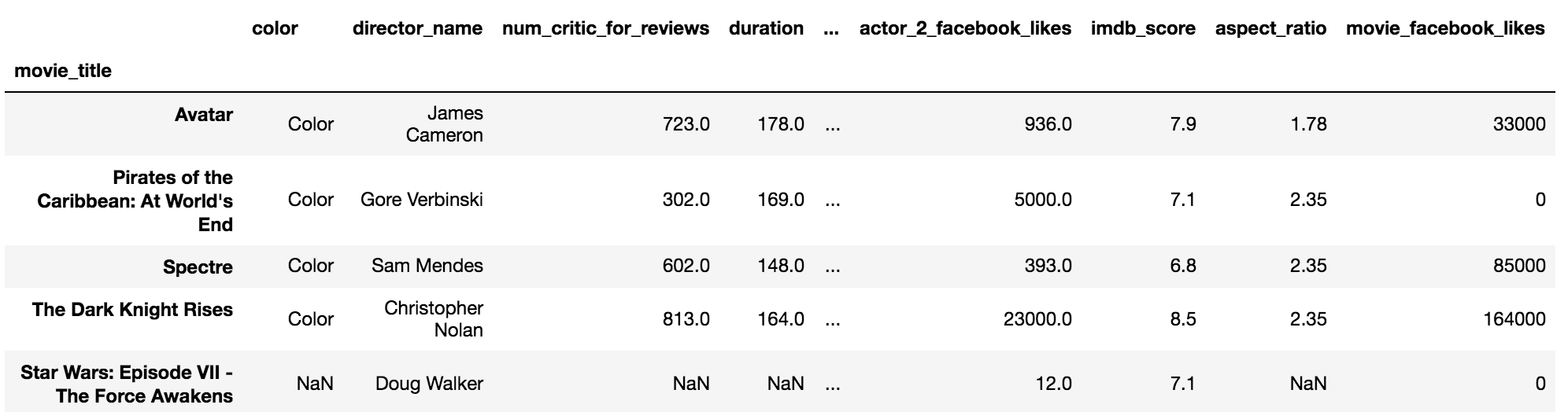
- Use the read_csv function to read in the movie dataset, and display the first five rows with the head method:
>>> movie = pd.read_csv('data/movie.csv')
>>> movie.head()
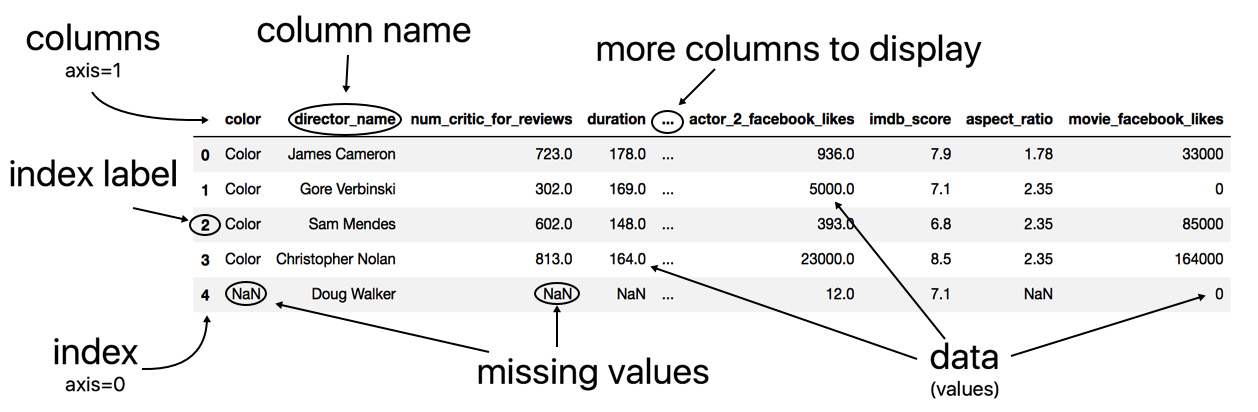
- Analyze the labeled anatomy of the DataFrame:
How it works...
Pandas first reads the data from disk into memory and into a DataFrame using the excellent and versatile read_csv function. The output for both the columns and the index is in bold font, which makes them easy to identify. By convention, the terms index label and column name refer to the individual members of the index and columns, respectively. The term index refers to all the index labels as a whole just as the term columns refers to all the column names as a whole.
The columns and the index serve a particular purpose, and that is to provide labels for the columns and rows of the DataFrame. These labels allow for direct and easy access to different subsets of data. When multiple Series or DataFrames are combined, the indexes align first before any calculation occurs. Collectively, the columns and the index are known as the axes.
DataFrame data (values) is always in regular font and is an entirely separate component from the columns or index. Pandas uses NaN (not a number) to represent missing values. Notice that even though the color column has only string values, it uses NaN to represent a missing value.
The three consecutive dots in the middle of the columns indicate that there is at least one column that exists but is not displayed due to the number of columns exceeding the predefined display limits.
There's more...
The head method accepts a single parameter, n, which controls the number of rows displayed. Similarly, the tail method returns the last n rows.
See also
- Pandas official documentation of the read_csv function (http://bit.ly/2vtJQ9A)
Accessing the main DataFrame components
Each of the three DataFrame components--the index, columns, and data--may be accessed directly from a DataFrame. Each of these components is itself a Python object with its own unique attributes and methods. It will often be the case that you would like to perform operations on the individual components and not on the DataFrame as a whole.
Getting ready
This recipe extracts the index, columns, and the data of the DataFrame into separate variables, and then shows how the columns and index are inherited from the same object.
How to do it...
- Use the DataFrame attributes index, columns, and values to assign the index, columns, and data to their own variables:
>>> movie = pd.read_csv('data/movie.csv')
>>> index = movie.index
>>> columns = movie.columns
>>> data = movie.values
- Display each component's values:
>>> index
RangeIndex(start=0, stop=5043, step=1)

>>> columns
Index(['color', 'director_name', 'num_critic_for_reviews',
       ...
       'imdb_score', 'aspect_ratio', 'movie_facebook_likes'],
       dtype='object')

>>> data
array([['Color', 'James Cameron', 723.0, ..., 7.9, 1.78, 33000],
       ...,
       ['Color', 'Jon Gunn', 43.0, ..., 6.6, 1.85, 456]],
       dtype=object)
- Output the type of each DataFrame component. The name of the type is the word following the last dot of the output:
>>> type(index)
pandas.core.indexes.range.RangeIndex

>>> type(columns)
pandas.core.indexes.base.Index

>>> type(data)
numpy.ndarray
- Interestingly, both the types for both the index and the columns appear to be closely related. The built-in issubclass method checks whether RangeIndex is indeed a subclass of Index:
>>> issubclass(pd.RangeIndex, pd.Index)
True
How it works...
You may access the three main components of a DataFrame with the index, columns, and values attributes. The output of the columns attribute appears to be just a sequence of the column names. This sequence of column names is technically an Index object. The output of the function type is the fully qualified class name of the object.
The built-in subclass function checks whether the first argument inherits from the second. The Index and RangeIndex objects are very similar, and in fact, pandas has a number of similar objects reserved specifically for either the index or the columns. The index and the columns must both be some kind of Index object. Essentially, the index and the columns represent the same thing, but along different axes. They’re occasionally referred to as the row index and column index.
A RangeIndex is a special type of Index object that is analogous to Python's range object. Its entire sequence of values is not loaded into memory until it is necessary to do so, thereby saving memory. It is completely defined by its start, stop, and step values.
There's more...
When possible, Index objects are implemented using hash tables that allow for very fast selection and data alignment. They are similar to Python sets in that they support operations such as intersection and union, but are dissimilar because they are ordered with duplicates allowed.
Notice how the values DataFrame attribute returned a NumPy n-dimensional array, or ndarray. Most of pandas relies heavily on the ndarray. Beneath the index, columns, and data are NumPy ndarrays. They could be considered the base object for pandas that many other objects are built upon. To see this, we can look at the values of the index and columns:
>>> index.values
array([   0,    1,    2, ..., 4913, 4914, 4915])

>>> columns.values
array(['color', 'director_name', 'num_critic_for_reviews',
 ...
 'imdb_score', 'aspect_ratio', 'movie_facebook_likes'],
 dtype=object)
See also
- Pandas official documentation of Indexing and Selecting data (http://bit.ly/2vm8f12)
- A look inside pandas design and development slide deck from pandas author, Wes McKinney (http://bit.ly/2u4YVLi)
Understanding data types
In very broad terms, data may be classified as either continuous or categorical. Continuous data is always numeric and represents some kind of measurement, such as height, wage, or salary. Continuous data can take on an infinite number of possibilities. Categorical data, on the other hand, represents discrete, finite amounts of values such as car color, type of poker hand, or brand of cereal.
Pandas does not broadly classify data as either continuous or categorical. Instead, it has precise technical definitions for many distinct data types. The following table contains all pandas data types, with their string equivalents, and some notes on each type:
| Common data type name | NumPy/pandas object | Pandas string name | Notes |
|
Boolean |
np.bool
|
bool |
Stored as a single byte. |
|
Integer |
np.int
|
int |
Defaulted to 64 bits. Unsigned ints are also available - np.uint. |
|
Float |
np.float |
float |
Defaulted to 64 bits. |
|
Complex |
np.complex |
complex |
Rarely seen in data analysis. |
|
Object |
np.object |
O, object |
Typically strings but is a catch-all for columns with multiple different types or other Python objects (tuples, lists, dicts, and so on). |
|
Datetime |
np.datetime64, pd.Timestamp |
datetime64 |
Specific moment in time with nanosecond precision. |
|
Timedelta |
np.timedelta64, pd.Timedelta |
timedelta64 |
An amount of time, from days to nanoseconds. |
|
Categorical |
pd.Categorical |
category |
Specific only to pandas. Useful for object columns with relatively few unique values. |
Getting ready
In this recipe, we display the data type of each column in a DataFrame. It is crucial to know the type of data held in each column as it fundamentally changes the kind of operations that are possible with it.
How to do it...
- Use the dtypes attribute to display each column along with its data type:
>>> movie = pd.read_csv('data/movie.csv')
>>> movie.dtypes
color                       object
director_name               object
num_critic_for_reviews     float64
duration                   float64
director_facebook_likes    float64
                            ...
title_year                 float64
actor_2_facebook_likes     float64
imdb_score                 float64
aspect_ratio               float64
movie_facebook_likes         int64
Length: 28, dtype: object
- Use the get_dtype_counts method to return the counts of each data type:
>>> movie.get_dtype_counts()
float64    13
int64       3
object     12
How it works...
Each DataFrame column must be exactly one type. For instance, every value in the column aspect_ratio is a 64-bit float, and every value in movie_facebook_likes is a 64-bit integer. Pandas defaults its core numeric types, integers, and floats to 64 bits regardless of the size necessary for all data to fit in memory. Even if a column consists entirely of the integer value 0, the data type will still be int64. get_dtype_counts is a convenience method for directly returning the count of all the data types in the DataFrame.
The object data type is the one data type that is unlike the others. A column that is of object data type may contain values that are of any valid Python object. Typically, when a column is of the object data type, it signals that the entire column is strings. This isn't necessarily the case as it is possible for these columns to contain a mixture of integers, booleans, strings, or other, even more complex Python objects such as lists or dictionaries. The object data type is a catch-all for columns that pandas doesn’t recognize as any other specific type.
There's more...
Almost all of pandas data types are built directly from NumPy. This tight integration makes it easier for users to integrate pandas and NumPy operations. As pandas grew larger and more popular, the object data type proved to be too generic for all columns with string values. Pandas created its own categorical data type to handle columns of strings (or numbers) with a fixed number of possible values.
See also
- Pandas official documentation for dtypes (http://bit.ly/2vxe8ZI)
- NumPy official documentation for Data types (http://bit.ly/2wq0qEH)
Selecting a single column of data as a Series
A Series is a single column of data from a DataFrame. It is a single dimension of data, composed of just an index and the data.
Getting ready
This recipe examines two different syntaxes to select a Series, one with the indexing operator and the other using dot notation.
How to do it...
- Pass a column name as a string to the indexing operator to select a Series of data:
>>> movie = pd.read_csv('data/movie.csv')
>>> movie['director_name']
- Alternatively, you may use the dot notation to accomplish the same task:
>>> movie.director_name
- Inspect the Series anatomy:

- Verify that the output is a Series:
>>> type(movie['director_name'])
pandas.core.series.Series
How it works...
Python has several built-in objects for containing data, such as lists, tuples, and dictionaries. All three of these objects use the indexing operator to select their data. DataFrames are more powerful and complex containers of data, but they too use the indexing operator as the primary means to select data. Passing a single string to the DataFrame indexing operator returns a Series.
The visual output of the Series is less stylized than the DataFrame. It represents a single column of data. Along with the index and values, the output displays the name, length, and data type of the Series.
Alternatively, while not recommended and subject to error, a column of data may be accessed using the dot notation with the column name as an attribute. Although it works with this particular example, it is not best practice and is prone to error and misuse. Column names with spaces or special characters cannot be accessed in this manner. This operation would have failed if the column name was director name. Column names that collide with DataFrame methods, such as count, also fail to be selected correctly using the dot notation. Assigning new values or deleting columns with the dot notation might give unexpected results. Because of this, using the dot notation to access columns should be avoided with production code.
There's more...
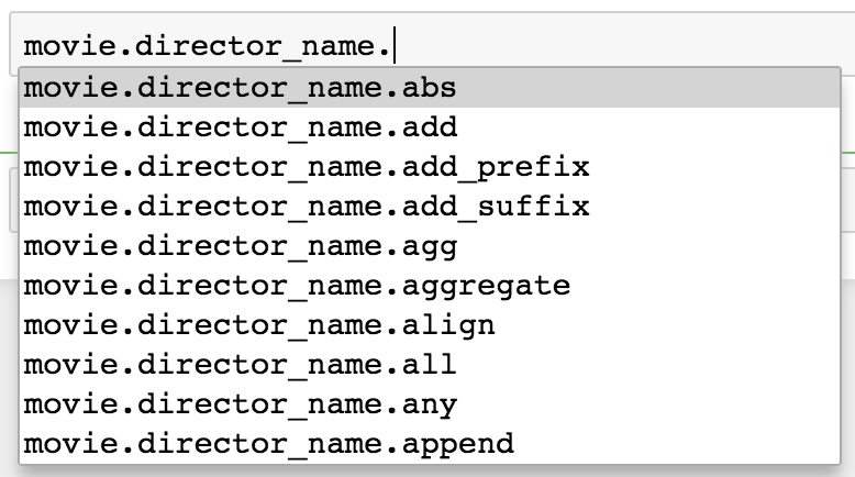
Why would anyone ever use the dot notation syntax if it causes trouble? Programmers are lazy, and there are fewer characters to type. But mainly, it is extremely handy when you want to have the autocomplete intelligence available. For this reason, column selection by dot notation will sometimes be used in this book. The autocomplete intelligence is fantastic for helping you become aware of all the possible attributes and methods available to an object.
The intelligence will fail to work when attempting to chain an operation after use of the indexing operator from step 1 but will continue to work with the dot notation from step 2. The following screenshot shows the pop-up window that appears after the selection of the director_name with the dot notation. All the possible attributes and methods will appear in a list after pressing Tab following the dot:
Yet another reason to be aware of the dot notation is the proliferation of its use online at the popular question and answer site Stack Overflow. Also, notice that the old column name is now the name of the Series and has actually become an attribute:
>>> director = movie['director_name']
>>> director.name
'director_name'
It is possible to turn this Series into a one-column DataFrame with the to_frame method. This method will use the Series name as the new column name:
>>> director.to_frame()
See also
- To understand how Python objects gain the capability to use the indexing operator, see the Python documentation on the __getitem__ special method (http://bit.ly/2u5ISN6)
- Refer to the Selecting multiple DataFrame columns recipe from Chapter 2, Essential DataFrame operations
Calling Series methods
Utilizing the single-dimensional Series is an integral part of all data analysis with pandas. A typical workflow will have you going back and forth between executing statements on Series and DataFrames. Calling Series methods is the primary way to use the abilities that the Series offers.
Getting ready
Both Series and DataFrames have a tremendous amount of power. We can use the dir function to uncover all the attributes and methods of a Series. Additionally, we can find the number of attributes and methods common to both Series and DataFrames. Both of these objects share the vast majority of attribute and method names:
>>> s_attr_methods = set(dir(pd.Series))
>>> len(s_attr_methods)
442

>>> df_attr_methods = set(dir(pd.DataFrame))
>>> len(df_attr_methods)
445

>>> len(s_attr_methods & df_attr_methods)
376
This recipe covers the most common and powerful Series methods. Many of the methods are nearly equivalent for DataFrames.
How to do it...
- After reading in the movies dataset, let's select two Series with different data types. The director_name column contains strings, formally an object data type, and the column actor_1_facebook_likes contains numerical data, formally float64:
>>> movie = pd.read_csv('data/movie.csv')
>>> director = movie['director_name']
>>> actor_1_fb_likes = movie['actor_1_facebook_likes']
- Inspect the head of each Series:
>>> director.head()
0        James Cameron
1       Gore Verbinski
2           Sam Mendes
3    Christopher Nolan
4          Doug Walker
Name: director_name, dtype: object

>>> actor_1_fb_likes.head()
0     1000.0
1    40000.0
2    11000.0
3    27000.0
4      131.0
Name: actor_1_facebook_likes, dtype: float64
- The data type of the Series usually determines which of the methods will be the most useful. For instance, one of the most useful methods for the object data type Series is value_counts, which counts all the occurrences of each unique value:
>>> director.value_counts()
Steven Spielberg        26
Woody Allen             22
Martin Scorsese         20
Clint Eastwood          20
                        ..
Fatih Akin               1
Analeine Cal y Mayor     1
Andrew Douglas           1
Scott Speer              1
Name: director_name, Length: 2397, dtype: int64
- The value_counts method is typically more useful for Series with object data types but can occasionally provide insight into numeric Series as well. Used with actor_1_fb_likes, it appears that higher numbers have been rounded to the nearest thousand as it is unlikely that so many movies received exactly 1,000 likes:
>>> actor_1_fb_likes.value_counts()
1000.0     436
11000.0    206
2000.0     189
3000.0     150
          ...
216.0        1
859.0        1
225.0        1
334.0        1
Name: actor_1_facebook_likes, Length: 877, dtype: int64
- Counting the number of elements in the Series may be done with the size or shape parameter or the len function:
>>> director.size
4916
>>> director.shape
(4916,)
>>> len(director)
4916
- Additionally, there is the useful but confusing count method that returns the number of non-missing values:
>>> director.count()
4814
>>> actor_1_fb_likes.count()
4909
- Basic summary statistics may be yielded with the min, max, mean, median, std, and sum methods:
>>> actor_1_fb_likes.min(), actor_1_fb_likes.max(), \
    actor_1_fb_likes.mean(), actor_1_fb_likes.median(), \
    actor_1_fb_likes.std(), actor_1_fb_likes.sum()
(0.0, 640000.0, 6494.488490527602, 982.0, 15106.98, 31881444.0)
- To simplify step 7, you may use the describe method to return both the summary statistics and a few of the quantiles at once. When describe is used with an object data type column, a completely different output is returned:
>>> actor_1_fb_likes.describe()
count      4909.000000
mean       6494.488491
std       15106.986884
min           0.000000
25%         607.000000
50%         982.000000
75%       11000.000000
max      640000.000000
Name: actor_1_facebook_likes, dtype: float64

>>> director.describe()
count                 4814
unique                2397
top       Steven Spielberg
freq                    26
Name: director_name, dtype: object
- The quantile method exists to calculate an exact quantile of numeric data:
>>> actor_1_fb_likes.quantile(.2)
510

>>> actor_1_fb_likes.quantile([.1, .2, .3, .4, .5,
                               .6, .7, .8, .9])
0.1      240.0
0.2      510.0
0.3      694.0
0.4      854.0
        ...
0.6     1000.0
0.7     8000.0
0.8    13000.0
0.9    18000.0
Name: actor_1_facebook_likes, Length: 9, dtype: float64
- Since the count method in step 6 returned a value less than the total number of Series elements found in step 5, we know that there are missing values in each Series. The isnull method may be used to determine whether each individual value is missing or not. The result will be a Series of booleans the same length as the original Series:
>>> director.isnull()
0       False
1       False
2       False
3       False
        ...
4912     True
4913    False
4914    False
4915    False
Name: director_name, Length: 4916, dtype: bool
- It is possible to replace all missing values within a Series with the fillna method:
>>> actor_1_fb_likes_filled = actor_1_fb_likes.fillna(0)
>>> actor_1_fb_likes_filled.count()
4916
- To remove the Series elements with missing values, use dropna:
>>> actor_1_fb_likes_dropped = actor_1_fb_likes.dropna()
>>> actor_1_fb_likes_dropped.size
4909
How it works...
Passing a string to the indexing operator of a DataFrame selects a single column as a Series. The methods used in this recipe were chosen because of how frequently they are used in data analysis.
The steps in this recipe should be straightforward with easily interpretable output. Even though the output is easy to read, you might lose track of the returned object. Is it a scalar value, a tuple, another Series, or some other Python object? Take a moment, and look at the output returned after each step. Can you name the returned object?
The result from the head method in step 1 is another Series. The value_counts method also produces a Series but has the unique values from the original Series as the index and the count as its values. In step 5, size and count return scalar values, but shape returns a one-item tuple.
In step 7, each individual method returns a scalar value, and is outputted as a tuple. This is because Python treats an expression composed of only comma-separated values without parentheses as a tuple.
In step 8, describe returns a Series with all the summary statistic names as the index and the actual statistic as the values.
In step 9, quantile is flexible and returns a scalar value when passed a single value but returns a Series when given a list.
From steps 10, 11, and 12, isnull, fillna, and dropna all return a Series.
There's more...
The value_counts method is one of the most informative Series methods and heavily used during exploratory analysis, especially with categorical columns. It defaults to returning the counts, but by setting the normalize parameter to True, the relative frequencies are returned instead, which provides another view of the distribution:
>>> director.value_counts(normalize=True)
Steven Spielberg        0.005401
Woody Allen             0.004570
Martin Scorsese         0.004155
Clint Eastwood          0.004155
                          ...
Fatih Akin              0.000208
Analeine Cal y Mayor    0.000208
Andrew Douglas          0.000208
Scott Speer             0.000208
Name: director_name, Length: 2397, dtype: float64
In this recipe, we determined that there were missing values in the Series by observing that the result from the count method did not match the size attribute. A more direct approach is to use the hasnans attribute:
>>> director.hasnans
True
There exists a complement of isnull: the notnull method, which returns True for all the non-missing values:
>>> director.notnull()
0        True
1        True
2        True
3        True
        ...
4912    False
4913     True
4914     True
4915     True
Name: director_name, Length: 4916, dtype: bool
See also
- To call many Series methods in succession, refer to the Chaining Series methods together recipe in this chapter
Working with operators on a Series
There exist a vast number of operators in Python for manipulating objects. Operators are not objects themselves, but rather syntactical structures and keywords that force an operation to occur on an object. For instance, when the plus operator is placed between two integers, Python will add them together. See more examples of operators in the following code:
>>> 5 + 9   # plus operator example adds 5 and 9
14

>>> 4 ** 2  # exponentiation operator raises 4 to the second power
16

>>> a = 10  # assignment operator assigns 10 to a

>>> 5 <= 9  # less than or equal to operator returns a boolean
True
Operators can work for any type of object, not just numerical data. These examples show different objects being operated on:
>>> 'abcde' + 'fg'
'abcdefg'

>>> not (5 <= 9)
False

>>> 7 in [1, 2, 6]
False

>>> set([1,2,3]) & set([2,3,4])
set([2,3])
Visit tutorials point (http://bit.ly/2u5g5Io) to see a table of all the basic Python operators. Not all operators are implemented for every object. These examples all produce errors when using an operator:
>>> [1, 2, 3] - 3
TypeError: unsupported operand type(s) for -: 'list' and 'int'

>>> a = set([1,2,3])
>>> a[0]
TypeError: 'set' object does not support indexing
Series and DataFrame objects work with most of the Python operators.
Getting ready
In this recipe, a variety of operators will be applied to different Series objects to produce a new Series with completely different values.
How to do it...
- Select the imdb_score column as a Series:
>>> movie = pd.read_csv('data/movie.csv')
>>> imdb_score = movie['imdb_score']
>>> imdb_score
0       7.9
1       7.1
2       6.8
       ...
4913    6.3
4914    6.3
4915    6.6
Name: imdb_score, Length: 4916, dtype: float64
- Use the plus operator to add one to each Series element:
>>> imdb_score + 1
0       8.9
1       8.1
2       7.8
       ...
4913    7.3
4914    7.3
4915    7.6
Name: imdb_score, Length: 4916, dtype: float64
- The other basic arithmetic operators minus (-), multiplication (*), division (/), and exponentiation (**) work similarly with scalar values. In this step, we will multiply the series by 2.5:
>>> imdb_score * 2.5
0       19.75
1       17.75
2       17.00
        ...
4913    15.75
4914    15.75
4915    16.50
Name: imdb_score, Length: 4916, dtype: float64
- Python uses two consecutive division operators (//) for floor division and the percent sign (%) for the modulus operator, which returns the remainder after a division. Series use these the same way:
>>> imdb_score // 7
0       1.0
1       1.0
2       0.0
       ...
4913    0.0
4914    0.0
4915    0.0
Name: imdb_score, Length: 4916, dtype: float64
- There exist six comparison operators, greater than (>), less than (<), greater than or equal to (>=), less than or equal to (<=), equal to (==), and not equal to (!=). Each comparison operator turns each value in the Series to True or False based on the outcome of the condition:
>>> imdb_score > 7
0        True
1        True
2       False
        ...
4913    False
4914    False
4915    False
Name: imdb_score, Length: 4916, dtype: bool

>>> director = movie['director_name']
>>> director == 'James Cameron'
0        True
1       False
2       False
        ...
4913    False
4914    False
4915    False
Name: director_name, Length: 4916, dtype: bool
How it works...
All the operators used in this recipe apply the same operation to each element in the Series. In native Python, this would require a for-loop to iterate through each of the items in the sequence before applying the operation. Pandas relies heavily on the NumPy library, which allows for vectorized computations, or the ability to operate on entire sequences of data without the explicit writing of for loops. Each operation returns a Series with the same index, but with values that have been modified by the operator.
There's more...
All of the operators used in this recipe have method equivalents that produce the exact same result. For instance, in step 1, imdb_score + 1 may be reproduced with the add method. Check the following code to see the method version of each step in the recipe:
>>> imdb_score.add(1)              # imdb_score + 1
>>> imdb_score.mul(2.5)            # imdb_score * 2.5
>>> imdb_score.floordiv(7)         # imdb_score // 7
>>> imdb_score.gt(7)               # imdb_score > 7
>>> director.eq('James Cameron')   # director == 'James Cameron'
Why does pandas offer a method equivalent to these operators? By its nature, an operator only operates in exactly one manner. Methods, on the other hand, can have parameters that allow you to alter their default functionality:
| Operator Group | Operator | Series method name |
| Arithmetic | +, -, *, /, //, %, ** | add, sub, mul, div, floordiv, mod, pow |
| Comparison | <, >, <=, >=, ==, != |
lt, gt, le, ge, eq, ne |
You may be curious as to how a Python Series object, or any object for that matter, knows what to do when it encounters an operator. For example, how does the expression imdb_score * 2.5 know to multiply each element in the Series by 2.5? Python has a built-in, standardized way for objects to communicate with operators using special methods.
Special methods are what objects call internally whenever they encounter an operator. Special methods are defined in the Python data model, a very important part of the official documentation, and are the same for every object throughout the language. Special methods always begin and end with two underscores. For instance, the special method __mul__ is called whenever the multiplication operator is used. Python interprets the imdb_score * 2.5 expression as imdb_score.__mul__(2.5).
There is no difference between using the special method and using an operator as they are doing the exact same thing. The operator is just syntactic sugar for the special method.
See also
- Python official documentation on operators (http://bit.ly/2wpOId8)
- Python official documentation on the data model (http://bit.ly/2v0LrDd)
Chaining Series methods together
In Python, every variable is an object, and all objects have attributes and methods that refer to or return more objects. The sequential invocation of methods using the dot notation is referred to as method chaining. Pandas is a library that lends itself well to method chaining, as many Series and DataFrame methods return more Series and DataFrames, upon which more methods can be called.
Getting ready
To motivate method chaining, let's take a simple English sentence and translate the chain of events into a chain of methods. Consider the sentence, A person drives to the store to buy food, then drives home and prepares, cooks, serves, and eats the food before cleaning the dishes.
A Python version of this sentence might take the following form:
>>> person.drive('store')\
          .buy('food')\
          .drive('home')\
          .prepare('food')\
          .cook('food')\
          .serve('food')\
          .eat('food')\
          .cleanup('dishes')
In the preceding code, the person is the object calling each of the methods, just as the person is performing all of the actions in the original sentence. The parameter passed to each of the methods specifies how the method operates.
Although it is possible to write the entire method chain in a single unbroken line, it is far more palatable to write a single method per line. Since Python does not normally allow a single expression to be written on multiple lines, you need to use the backslash line continuation character. Alternatively, you may wrap the whole expression in parentheses. To improve readability even more, place each method directly under the dot above it. This recipe shows similar method chaining with pandas Series.
How to do it...
- Load in the movie dataset, and select two columns as a distinct Series:
>>> movie = pd.read_csv('data/movie.csv')
>>> actor_1_fb_likes = movie['actor_1_facebook_likes']
>>> director = movie['director_name']
- One of the most common methods to append to the chain is the head method. This suppresses long output. For shorter chains, there isn't as great a need to place each method on a different line:
>>> director.value_counts().head(3)
Steven Spielberg    26
Woody Allen         22
Clint Eastwood      20
Name: director_name, dtype: int64
- A common way to count the number of missing values is to chain the sum method after isnull:
>>> actor_1_fb_likes.isnull().sum()
7
- All the non-missing values of actor_1_fb_likes should be integers as it is impossible to have a partial Facebook like. Any numeric columns with missing values must have their data type as float. If we fill missing values from actor_1_fb_likes with zeros, we can then convert it to an integer with the astype method:
>>> actor_1_fb_likes.dtype
dtype('float64')

>>> actor_1_fb_likes.fillna(0)\
                    .astype(int)\
                    .head()
0     1000
1    40000
2    11000
3    27000
4      131
Name: actor_1_facebook_likes, dtype: int64
How it works...
Method chaining is possible with all Python objects since each object method must return another object that itself will have more methods. It is not necessary for the method to return the same type of object.
Step 2 first uses value_counts to return a Series and then chains the head method to select the first three elements. The final returned object is a Series, which could also have had more methods chained on it.
In step 3, the isnull method creates a boolean Series. Pandas numerically evaluates False/True as 0/1, so the sum method returns the number of missing values.
Each of the three chained methods in step 4 returns a Series. It may not seem intuitive, but the astype method returns an entirely new Series with a different data type
There's more...
Instead of summing up the booleans in step 3 to find the total number of missing values, we can take the mean of the Series to get the percentage of values that are missing:
>>> actor_1_fb_likes.isnull().mean()
0.0014
As was mentioned at the beginning of the recipe, it is possible to use parentheses instead of the backslash for multi-line code. Step 4 may be rewritten this way:
>>> (actor_1_fb_likes.fillna(0)
                     .astype(int)
                     .head())
Not all programmers like the use of method chaining, as there are some downsides. One such downside is that debugging becomes difficult. None of the intermediate objects produced during the chain are stored in a variable, so if there is an unexpected result, it will be difficult to trace the exact location in the chain where it occurred.
The example at the start of the recipe may be rewritten so that the result of each method gets preserved as/in a unique variable. This makes tracking bugs much easier, as you can inspect the object at each step:
>>> person1 = person.drive('store')
>>> person2 = person1.buy('food')
>>> person3 = person2.drive('home')
>>> person4 = person3.prepare('food')
>>> person5 = person4.cook('food')
>>> person6 = person5.serve('food')
>>> person7 = person6.eat('food')
>>> person8 = person7.cleanup('dishes')
Making the index meaningful
The index of a DataFrame provides a label for each of the rows. If no index is explicitly provided upon DataFrame creation, then by default, a RangeIndex is created with labels as integers from 0 to n-1, where n is the number of rows.
Getting ready
This recipe replaces the meaningless default row index of the movie dataset with the movie title, which is much more meaningful.
How to do it...
- Read in the movie dataset, and use the set_index method to set the title of each movie as the new index:
>>> movie = pd.read_csv('data/movie.csv')
>>> movie2 = movie.set_index('movie_title')
>>> movie2
- Alternatively, it is possible to choose a column as the index upon initial read with the index_col parameter of the read_csv function:
>>> movie = pd.read_csv('data/movie.csv', index_col='movie_title')
How it works...
A meaningful index is one that clearly identifies each row. The default RangeIndex is not very helpful. Since each row identifies data for exactly one movie, it makes sense to use the movie title as the label. If you know ahead of time which column will make a good index, you can specify this upon import with the index_col parameter of the read_csv function.
By default, both set_index and read_csv drop the column used as the index from the DataFrame. With set_index, it is possible to keep the column in the DataFrame by setting the drop parameter to False.
There's more...
Conversely, it is possible to turn the index into a column with the reset_index method. This will make movie_title a column again and revert the index back to a RangeIndex. reset_index always puts the column as the very first one in the DataFrame, so the columns may not be in their original order:
>>> movie2.reset_index()
See also
- Pandas official documentation on RangeIndex (http://bit.ly/2hs6DNL)
Renaming row and column names
One of the most basic and common operations on a DataFrame is to rename the row or column names. Good column names are descriptive, brief, and follow a common convention with respect to capitalization, spaces, underscores, and other features.
Getting ready
In this recipe, both the row and column names are renamed.
How to do it...
- Read in the movie dataset, and make the index meaningful by setting it as the movie title:
>>> movie = pd.read_csv('data/movie.csv', index_col='movie_title')
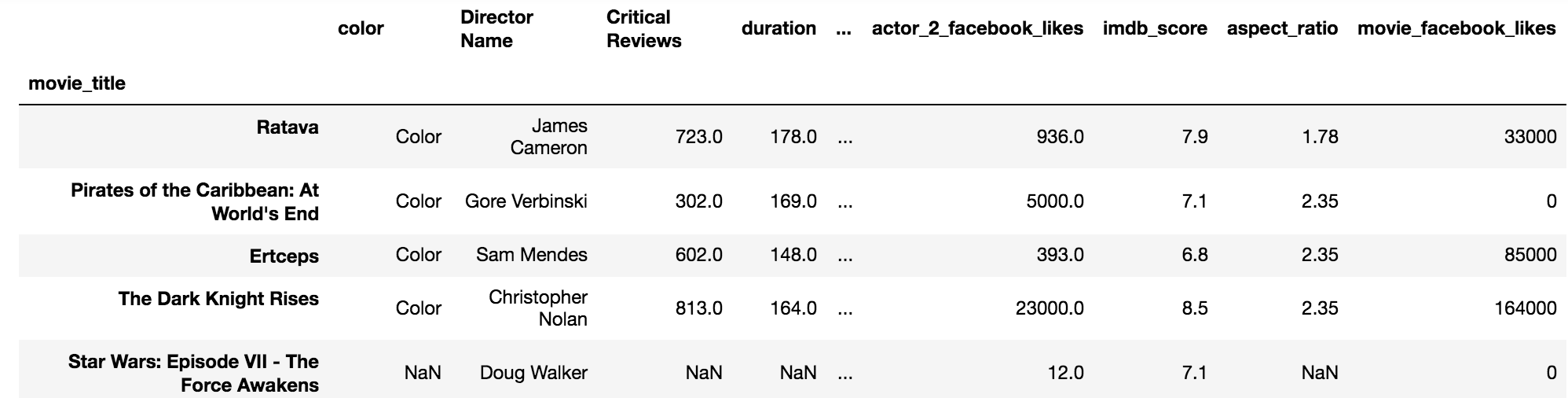
- The rename DataFrame method accepts dictionaries that map the old value to the new value. Let's create one for the rows and another for the columns:
>>> idx_rename = {'Avatar':'Ratava', 'Spectre': 'Ertceps'}
>>> col_rename = {'director_name':'Director Name',
                  'num_critic_for_reviews': 'Critical Reviews'}
- Pass the dictionaries to the rename method, and assign the result to a new variable:
>>> movie_renamed = movie.rename(index=idx_rename,
                                 columns=col_rename)
>>> movie_renamed.head()
How it works...
The rename DataFrame method allows for both row and column labels to be renamed at the same time with the index and columns parameters. Each of these parameters may be set to a dictionary that maps old labels to their new values.
There's more...
There are multiple ways to rename row and column labels. It is possible to reassign the index and column attributes directly to a Python list. This assignment works when the list has the same number of elements as the row and column labels. The following code uses the tolist method on each Index object to create a Python list of labels. It then modifies a couple values in the list and reassigns the list to the attributes index and columns:
>>> movie = pd.read_csv('data/movie.csv', index_col='movie_title')
>>> index = movie.index
>>> columns = movie.columns

>>> index_list = index.tolist()
>>> column_list = columns.tolist()

# rename the row and column labels with list assignments
>>> index_list[0] = 'Ratava'
>>> index_list[2] = 'Ertceps'
>>> column_list[1] = 'Director Name'
>>> column_list[2] = 'Critical Reviews'

>>> print(index_list)
['Ratava', "Pirates of the Caribbean: At World's End", 'Ertceps', 'The Dark Knight Rises', ... ]

>>> print(column_list)
['color', 'Director Name', 'Critical Reviews', 'duration', ...]

# finally reassign the index and columns
>>> movie.index = index_list
>>> movie.columns = column_list
Creating and deleting columns
During a data analysis, it is extremely likely that you will need to create new columns to represent new variables. Commonly, these new columns will be created from previous columns already in the dataset. Pandas has a few different ways to add new columns to a DataFrame.
Getting ready
In this recipe, we create new columns in the movie dataset by using the assignment and then delete columns with the drop method.
How to do it...
- The simplest way to create a new column is to assign it a scalar value. Place the name of the new column as a string into the indexing operator. Let's create the has_seen column in the movie dataset to indicate whether or not we have seen the movie. We will assign zero for every value. By default, new columns are appended to the end:
>>> movie = pd.read_csv('data/movie.csv')
>>> movie['has_seen'] = 0
- There are several columns that contain data on the number of Facebook likes. Let's add up all the actor and director Facebook likes and assign them to the actor_director_facebook_likes column:
>>> movie['actor_director_facebook_likes'] =  \
        (movie['actor_1_facebook_likes'] +
         movie['actor_2_facebook_likes'] +
         movie['actor_3_facebook_likes'] +
         movie['director_facebook_likes'])
- From the Calling Series method recipe in this chapter, we know that this dataset contains missing values. When numeric columns are added to one another as in the preceding step, pandas defaults missing values to zero. But, if all values for a particular row are missing, then pandas keeps the total as missing as well. Let's check if there are missing values in our new column and fill them with 0:
>>> movie['actor_director_facebook_likes'].isnull().sum()
122
>>> movie['actor_director_facebook_likes'] = \
    movie['actor_director_facebook_likes'].fillna(0)
- There is another column in the dataset named cast_total_facebook_likes. It would be interesting to see what percentage of this column comes from our newly created column, actor_director_facebook_likes. Before we create our percentage column, let's do some basic data validation. Let's ensure that cast_total_facebook_likes is greater than or equal to actor_director_facebook_likes:
>>> movie['is_cast_likes_more'] = \
         (movie['cast_total_facebook_likes'] >=
          movie['actor_director_facebook_likes'])
- is_cast_likes_more is now a column of boolean values. We can check whether all the values of this column are True with the all Series method:
>>> movie['is_cast_likes_more'].all()
False
- It turns out that there is at least one movie with more actor_director_facebook_likes than cast_total_facebook_likes. It could be that director Facebook likes are not part of the cast total likes. Let's backtrack and delete column actor_director_facebook_likes:
>>> movie = movie.drop('actor_director_facebook_likes',
                       axis='columns')
- Let's recreate a column of just the total actor likes:
>>> movie['actor_total_facebook_likes'] = \
         (movie['actor_1_facebook_likes'] +
          movie['actor_2_facebook_likes'] +
          movie['actor_3_facebook_likes'])

>>> movie['actor_total_facebook_likes'] = \
         movie['actor_total_facebook_likes'].fillna(0)
- Check again whether all the values in cast_total_facebook_likes are greater than the actor_total_facebook_likes:
>>> movie['is_cast_likes_more'] = \
         (movie['cast_total_facebook_likes'] >=
          movie['actor_total_facebook_likes'])

>>> movie['is_cast_likes_more'].all()
True
- Finally, let's calculate the percentage of the cast_total_facebook_likes that come from actor_total_facebook_likes:
>>> movie['pct_actor_cast_like'] = \
         (movie['actor_total_facebook_likes'] /
          movie['cast_total_facebook_likes'])
- Let's validate that the min and max of this column fall between 0 and 1:
>>> (movie['pct_actor_cast_like'].min(),
     movie['pct_actor_cast_like'].max())
(0.0, 1.0)
- We can then output this column as a Series. First, we need to set the index to the movie title so we can properly identify each value.
>>> movie.set_index('movie_title')['pct_actor_cast_like'].head()
movie_title
Avatar                                        0.577369
Pirates of the Caribbean: At World's End      0.951396
Spectre                                       0.987521
The Dark Knight Rises                         0.683783
Star Wars: Episode VII - The Force Awakens    0.000000
Name: pct_actor_cast_like, dtype: float64
How it works...
Many pandas operations are flexible, and column creation is one of them. This recipe assigns both a scalar value, as seen in Step 1, and a Series, as seen in step 2, to create a new column.
Step 2 adds four different Series together with the plus operator. Step 3 uses method chaining to find and fill missing values. Step 4 uses the greater than or equal comparison operator to return a boolean Series, which is then evaluated with the all method in step 5 to check whether every single value is True or not.
The drop method accepts the name of the row or column to delete. It defaults to dropping rows by the index names. To drop columns you must set the axis parameter to either 1 or columns. The default value for axis is 0 or the string index.
Steps 7 and 8 redo the work of step 3 to step 5 without the director_facebook_likes column. Step 9 finally calculates the desired column we wanted since step 4. Step 10 validates that the percentages are between 0 and 1.
There's more...
It is possible to insert a new column into a specific place in a DataFrame besides the end with the insert method. The insert method takes the integer position of the new column as its first argument, the name of the new column as its second, and the values as its third. You will need to use the get_loc Index method to find the integer location of the column name.
The insert method modifies the calling DataFrame in-place, so there won't be an assignment statement. The profit of each movie may be calculated by subtracting budget from gross and inserting it directly after gross with the following:
>>> profit_index = movie.columns.get_loc('gross') + 1
>>> profit_index
9

>>> movie.insert(loc=profit_index,
                 column='profit',
                 value=movie['gross'] - movie['budget'])
An alternative to deleting columns with the drop method is to use the del statement:
>>> del movie['actor_director_facebook_likes']