Research consistently shows that machine learning and data science practitioners spend most of their time manipulating data and preparing it for analysis. Indeed, many find it the most tedious and least enjoyable part of their work. Numerous companies are offering solutions to the problem but, in my opinion, results at this point are varied. Therefore, in this first chapter, I shall endeavor to provide a way of tackling the problem that will ease the burden of getting your data ready for machine learning. The methodology introduced in this chapter will serve as the foundation for data preparation and for understanding many of the subsequent chapters. I propose that once you become comfortable with this tried and true process, it may very well become your favorite part of machine learning—as it is for me.

The following are the topics that we'll cover in this chapter:

• Overview
• Reading the data
• Handling duplicate observations
• Descriptive statistics
• Exploring categorical variables
• Handling missing values
• Zero and near-zero variance features
• Treating the data
• Correlation and linearity

If you haven't been exposed to large, messy datasets, then be patient, for it's only a matter of time. If you've encountered such data, has it been in a domain where you have little subject matter expertise? If not, then once again I proffer that it's only a matter of time. Some of the common problems that make up this term messy data include the following:

• Missing or invalid values
• Novel levels in a categorical feature that show up in algorithm production
• High cardinality in categorical features such as zip codes
• High dimensionality
• Duplicate observations

So this begs the question what are we to do? Well, first we need to look at what are the critical tasks that need to be performed during this phase of the process. The following tasks serve as the foundation for building a learning algorithm. They're from the paper by SPSS, CRISP-DM 1.0, a step-by-step data-mining guide available at https://the-modeling-agency.com/crisp-dm.pdf:

• Data understanding:
  1. Collect
  2. Describe
  3. Explore
  4. Verify
• Data preparation:
  1. Select
  2. Clean
  3. Construct
  4. Integrate
  5. Format

Certainly this is an excellent enumeration of the process, but what do we really need to do? I propose that, in practical terms we can all relate to, the following must be done once the data is joined and loaded into your machine, cloud, or whatever you use:

• Understand the data structure
• Dedupe observations
• Eliminate zero variance features and low variance features as desired
• Handle missing values
• Create dummy features (one-hot encoding)
• Examine and deal with highly correlated features and those with perfect linear relationships
• Scale as necessary
• Create other features as desired

Many feel that this is a daunting task. I don't and, in fact, I quite enjoy it. If done correctly and with a judicious application of judgment, it should reduce the amount of time spent at this first stage of a project and facilitate training your learning algorithm. None of the previous steps are challenging, but it can take quite a bit of time to write the code to perform each task.

Well, that's the benefit of this chapter. The example to follow will walk you through the tasks and the R code that accomplishes it. The code is flexible enough that you should be able to apply it to your projects. Additionally, it will help you gain an understanding of the data at a point you can intelligently discuss it with Subject Matter Experts (SMEs) if, in fact, they're available.

In the practical exercise that follows, we'll work with a small dataset. However, it suffers from all of the problems described earlier. Don't let the small size fool you, as we'll take what we learn here and use it for the more massive datasets to come in subsequent chapters.

As background, the data we'll use I put together painstakingly by hand. It's the Order of Battle for the opposing armies at the Battle of Gettysburg, fought during the American Civil War, July 1^st-3^rd, 1863, and the casualties reported by the end of the day on July 3^rd. I purposely chose this data because I'm reasonably sure you know very little about it. Don't worry, I'm the SME on the battle here and will walk you through it every step of the way. The one thing that we won't cover in this chapter is dealing with large volumes of textual features, which we'll discuss later in this book. Enough said already; let's get started!

This first task will load the data and show how to get a how level understanding of its structure and dimensions as well as install the necessary packages.

You have two ways to access the data, which resides on GitHub. You can download gettysburg.csv directly from the site at this link: https://github.com/datameister66/MMLR3rd, or you can use the RCurl package. An example of how to use the package is available here: https://github.com/opetchey/RREEBES/wiki/Reading-data-and-code-from-an-online-github-repository.

Let's assume you have the file in your working directory, so let's begin by installing the necessary packages:

install.packages("caret")
install.packages("janitor")
install.packages("readr")
install.packages("sjmisc")
install.packages("skimr")
install.packages("tidyverse")
install.packages("vtreat")

Let me make a quick note about how I've learned (the hard way) about how to correctly write code. With the packages installed, we could now specifically call the libraries into the R environment. However, it's a best practice and necessary when putting code into production that a function that isn't in base R be specified. First, this helps you and unfortunate others to read your code with an understanding of which library is mapped to a specific function. It also eliminates potential errors because different packages call different functions the same thing. The example that comes to my mind is the tsoutliers() function. The function is available in the forecast package and was in the tsoutliers package during earlier versions. Now I know this extra typing might seem unwieldy and unnecessary, but once you discipline yourself to do it, you'll find that it's well worth the effort.

There's one library we'll call and that's magrittr, which allows the use of a pipe-operator, %>%, to chain code together:

library(magrittr)

We're now ready to load the .csv file. In doing so, let's utilize the read_csv() function from readr as it's faster than base R and creates a tibble dataframe. In most cases, using tibbles in a tidyverse style is easier to write and understand. If you want to learn all the benefits of tidyverse, check out their website: tidyverse.org.

The only thing we need to specify in the function is our filename:

gettysburg <- read_csv("~/gettysburg.csv")

Here's a look at the column (feature) names:

colnames(gettysburg)
[1]  "type"           "state"          "regiment_or_battery" "brigade"
[5]  "division"       "corps"          "army"                "july1_Commander"
[9]  "Cdr_casualty"   "men"            "killed"              "wounded"
[13] "captured"       "missing"        "total_casualties"    "3inch_rifles"
[17] "4.5inch_rifles" "10lb_parrots"   "12lb_howitzers"      "12lb_napoleons"
[21] "6lb_howitzers"  "24lb_howitzers" "20lb_parrots"        "12lb_whitworths"
[25] "14lb_rifles"    "total_guns"

We have 26 features in this data, and some of you're asking yourself things like, what the heck is a 20 pound parrot? If you put it in a search engine, you'll probably end up with the bird and not the 20 pound Parrot rifled artillery gun. You can see the dimensions of the data in RStudio in your Global Environment view, or you can dig on your own to see there're 590 observations:

dim(gettysburg)
[1] 590 26

So we have 590 observations of 26 features, but this data suffers from the issues that permeate large and complex data. Next, we'll explore if there're any duplicate observations and how to deal with them efficiently.

The easiest way to get started is to use the base R duplicated() function to create a vector of logical values that match the data observations. These values will consist of either TRUE or FALSE where TRUE indicates a duplicate. Then, we'll create a table of those values and their counts and identify which of the rows are dupes:

dupes <- duplicated(gettysburg)

table(dupes)
dupes
FALSE TRUE
  587    3

which(dupes == "TRUE")
[1] 588 589

To rid ourselves of these duplicate rows, we put the distinct() function for the dplyr package to good use, specifying .keep_all = TRUE to make sure we return all of the features into the new tibble. Note that .keep_all defaults to FALSE:

gettysburg <- dplyr::distinct(gettysburg, .keep_all = TRUE)

Notice that, in the Global Environment, the tibble is now a dimension of 587 observations of 26 variables/features.

With the duplicate observations out of the way, it's time to start drilling down into the data and understand its structure a little better by exploring the descriptive statistics of the quantitative features.

Traditionally, we could use the base R summary() function to identify some basic statistics. Now, and recently I might add, I like to use the package sjmisc and its descr() function. It produces a more readable output, and you can assign that output to a dataframe. What works well is to create that dataframe, save it as a .csv, and explore it at your leisure. It automatically selects numeric features only. It also fits well with tidyverse so that you can incorporate dplyr functions such as group_by() and filter(). Here's an example in our case where we examine the descriptive stats for the infantry of the Confederate Army. The output will consist of the following:

• var: feature name
• type: integer
• n: number of observations
• NA.prc: percent of missing values
• mean
• sd: standard deviation
• se: standard error
• md: median
• trimmed: trimmed mean
• range
• skew

gettysburg %>%
  dplyr::filter(army == "Confederate" & type == "Infantry") %>%
  sjmisc::descr() -> descr_stats

readr::write_csv(descr_stats, 'descr_stats.csv')

The following is abbreviated output from the preceding code saved to a spreadsheet:

In this one table, we can discern some rather interesting tidbits. In particular is the percent of missing values per feature. If you modify the precious code to examine the Union Army, you'll find that there're no missing values. The reason the usurpers from the South had missing values is based on a couple of factors; either shoddy staff work in compiling the numbers on July 3^rd or the records were lost over the years. Note that, for the number of men captured, if you remove the missing value, all other values are zero, so we could just replace the missing value with it. The Rebels did not report troops as captured, but rather as missing, in contrast with the Union.

Once you feel comfortable with the descriptive statistics, move on to exploring the categorical features in the next section.

When it comes to an understanding of your categorical variables, there're many different ways to go about it. We can easily use the base R table() function on a feature. If you just want to see how many distinct levels are in a feature, then dplyr works well. In this example, we examine type, which has three unique levels:

dplyr::count(gettysburg, dplyr::n_distinct(type))

The output of the preceding code is as follows:

# A tibble: 1 x 2
     `dplyr::n_distinct(type)`        n
                                            <int> <int>
                                                     3    587

Let's now look at a way to explore all of the categorical features utilizing tidyverse principles. Doing it this way always allows you to save the tibble and examine the results in depth as needed. Here is a way of putting all categorical features into a separate tibble:

gettysburg_cat <-
  gettysburg[, sapply(gettysburg, class) == 'character']

Using dplyr, you can now summarize all of the features and the number of distinct levels in each:

gettysburg_cat %>%
  dplyr::summarise_all(dplyr::funs(dplyr::n_distinct(.)))

The output of the preceding code is as follows:

# A tibble: 1 x 9
   type  state regiment_or_battery brigade division corps  army july1_Commander  Cdr_casualty
 <int> <int>                                  <int>      <int>      <int> <int> <int>                            <int>                  <int>
          3       30                                      275           124            38        14          2                                586                           6

Notice that there're 586 distinct values to july1_Commander. This means that two of the unit Commanders have the same rank and last name. We can also surmise that this feature will be of no value to any further analysis, but we'll deal with that issue in a couple of sections ahead.

Suppose we're interested in the number of observations for each of the levels for the Cdr_casualty feature. Yes, we could use table(), but how about producing the output as a tibble as discussed before? Give this code a try:

gettysburg_cat %>% 
  dplyr::group_by(Cdr_casualty) %>%
  dplyr::summarize(num_rows = n())

The output of the preceding code is as follows:

# A tibble: 6 x 2
 Cdr_casualty                    num_rows
    <chr>                           <int>
 1 captured                            6
 2 killed                             29
 3 mortally wounded                   24
 4 no                                405
 5 wounded                           104
 6 wounded-captured                   19

Speaking of tables, let's look at a tibble-friendly way of producing one using two features. This code takes the idea of comparing commander casualties by army:

gettysburg_cat %>%
  janitor::tabyl(army, Cdr_casualty)

The output of the preceding code is as follows:

army   captured killed mortally wounded   no  wounded  wounded-captured
Confederate  2    15               13     165    44             17
Union        4    14               11     240    60              2

Explore the data on your own and, once you're comfortable with the categorical variables, let's tackle the issue of missing values.

Dealing with missing values can be a little tricky as there's a number of ways to approach the task. We've already seen in the section on descriptive statistics that there're missing values. First of all, let's get a full accounting of the missing quantity by feature, then we shall discuss how to deal with them. What I'm going to demonstrate in the following is how to put the count by feature into a dataframe that we can explore within RStudio:

na_count <-
  sapply(gettysburg, function(y)
    sum(length(which(is.na(
      y
    )))))

na_df <- data.frame(na_count)

View(na_df)

The following is a screenshot produced by the preceding code, after sorting the dataframe by descending count:

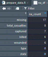
You can clearly see the count of missing by feature with the most missing is ironically named missing with a total of 17 observations.

So what should we do here or, more appropriately, what can we do here? There're several choices:

• Do nothing: However, some R functions will omit NAs and some functions will fail and produce an error.
• Omit all observations with NAs: In massive datasets, they may make sense, but we run the risk of losing information.
• Impute values: They could be something as simple as substituting the median value for the missing one or creating an algorithm to impute the values.
• Dummy coding: Turn the missing into a value such as 0 or -999, and code a dummy feature where if the feature for a specific observation is missing, the dummy is coded 1, otherwise, it's coded 0.

I could devote an entire chapter, indeed a whole book on the subject, delving into missing at random and others, but I was trained—and, in fact, shall insist—on the latter method. It's never failed me and the others can be a bit problematic. The benefit of dummy coding—or indicator coding, if you prefer—is that you don't lose information. In fact, missing-ness might be an essential feature in and of itself.

So, here's an example of how I manually code a dummy feature and turn the NAs into zeroes:

gettysburg$missing_isNA <- 
  ifelse(is.na(gettysburg$missing), 1, 0)

gettysburg$missing[is.na(gettysburg$missing)] <- 0

The first iteration of code creates a dummy feature for the missing feature and the second changes any NAs in missing to zero. In the upcoming section, where the dataset is fully processed (treated), the other missing values will be imputed.

Before moving on to dataset treatment, it's an easy task to eliminate features that have either one unique value (zero variance) or a high ratio of the most common value to the next most common value such that there're few unique values (near-zero variance). To do this, we'll lean on the caret package and the nearZeroVar() function. We get started by creating a dataframe and using the function's defaults except for saveMetrics = TRUE. We need to make that specification to return the dataframe:

feature_variance <- caret::nearZeroVar(gettysburg, saveMetrics = TRUE)

The output is quite interesting, so let's peek at the first six rows of what we produced:

head(feature_variance)

The output of the preceding code is as follows:

                       freqRatio     percentUnique    zeroVar     nzv
          type         3.186047      0.5110733        FALSE     FALSE
         state         1.094118      5.1107325        FALSE     FALSE
regiment_or_battery    1.105263     46.8483816        FALSE     FALSE
         brigade       1.111111     21.1243612        FALSE     FALSE
         division      1.423077      6.4735945        FALSE     FALSE
          corps        1.080000      2.3850085        FALSE     FALSE

The two key columns are zeroVar and nzv. They act as an indicator of whether or not that feature is zero variance or near-zero variance; TRUE indicates yes and FALSE not so surprisingly indicates no. The other columns must be defined:

• freqRatio: This is the ratio of the percentage frequency for the most common value over the second most common value.
• percentUnique: This is the number of unique values divided by the total number of samples multiplied by 100.

Let me explain that with the data we're using. For the type feature, the most common value is Infantry, which is roughly three times more common than Artillery. For percentUnique, the lower the percentage, the lower the number of unique values. You can explore this dataframe and adjust the function to determine your relevant cut points. For this example, we'll see whether we have any zero variance features by running this code:

which(feature_variance$zeroVar == 'TRUE')

The output of the preceding code is as follows:

[1] 17

Alas, we see that row 17 (feature 17) has zero variance. Let's see what that could be:

row.names(feature_variance[17, ])

The output of the preceding code is as follows:

[1] "4.5inch_rifles"

This is quite strange to me. What it means is that I failed to record the number of the artillery piece in the one Confederate unit that brought them to the battle. An egregious error on my part discovered using an elegant function from the caret package. Oh well, let's create a new tibble with this filtered out for demonstration purposes:

gettysburg_fltrd <- gettysburg[, feature_variance$zeroVar == 'FALSE']

This code eliminates the zero variance feature. If we wanted also to eliminate near-zero variance as well, just run the code and substitute feature_variance$zerVar with feature_variance$nzv.

We're now ready to perform the real magic of this process and treat our data.

What do I mean when I say let's treat the data? I learned the term from the authors of the vtreat package, Nina Zumel, and John Mount. You can read their excellent paper on the subject at this link: https://arxiv.org/pdf/1611.09477.pdf.

The definition they provide is: processor or conditioner that prepares real-world data for predictive modeling in a statistically sound manner. In treating your data, you'll rid yourself of many of the data preparation headaches discussed earlier. The example with our current dataset will provide an excellent introduction into the benefits of this method and how you can tailor it to your needs. I kind of like to think that treating your data is a smarter version of one-hot encoding.

The package offers three different functions to treat data, but I only use one and that is designTreatmentsZ(), which treats the features without regard to an outcome or response. The functions designTreatmentsC() and designTreatmentsN() functions build dataframes based on categorical and numeric outcomes respectively. Those functions provide a method to prune features in a univariate fashion. I'll provide other ways of conducting feature selection, so that's why I use that specific function. I encourage you to experiment on your own.

The function we use in the following will produce an object that you can apply to training, validation, testing, and even production data. In later chapters, we'll focus on training and testing, but here let's treat the entire data without considerations of any splits for simplicity. There're a number of arguments in the function you can change, but the defaults are usually sufficient. We'll specify the input data, the feature names to include, and minFraction, which is defined by the package as the optional minimum frequency a categorical level must have to be converted into an indicator column. I've chosen 5% and the minimum frequency. In real-world data, I've seen this number altered many times to find the right level of occurrence:

my_treatment <- vtreat::designTreatmentsZ(
  dframe = gettysburg_fltrd,
  varlist = colnames(gettysburg_fltrd),
  minFraction = 0.05
)

We now have an object with a stored treatment plan. Now we just use the prepare() function to apply that treatment to a dataframe or tibble, and it'll give us a treated dataframe:

gettysburg_treated <- vtreat::prepare(my_treatment, gettysburg_fltrd)

dim(gettysburg_treated)

The output of the preceding code is as follows:

[1]   587      54

We now have 54 features. Let's take a look at their names:

colnames(gettysburg_treated)

The abbreviated output of the preceding code is as follows:

[1]     "type_catP"       "state_catP"      "regiment_or_battery_catP"
[4]  "brigade_catP"    "division_catP"                    "corps_catP"

As you explore the names, you'll notice that we have features ending in catP, clean, and isBAD and others with _lev_x_ in them. Let's cover each in detail. As for catP features, the function creates a feature that's the frequency for the categorical level in that observation. What does that mean? Let's see a table for type_catP:

table(gettysburg_treated$type_catP)

The output of the preceding code is as follows:

0.080068143100   0.21976149914    0.70017035775
            47             129              411

This tells us that 47 rows are of category level x (in this case, Cavalry), and this is 8% of the total observations. As such, 22% are Artillery and 70% Infantry. This can be helpful in further exploring your data and to help adjust the minimum frequency in your category levels. I've heard it discussed that these values could help in the creation of a distance or similarity matrix.

The next is clean. These are our numeric features that have had missing values imputed, which is the feature mean, and outliers winsorized or collared if you specified the argument in the prepare() function. We didn't, so only missing values were imputed.

Speaking of missing values, this brings us to isBAD. This feature is the 1 for missing and 0 if not missing we talked about where I manually coded it.

Finally, lev_x is the dummy feature coding for a specific categorical level. If you go through the levels that were hot-encoded for states, you'll find features for Georgia, New York, North Carolina, Pennsylvania, US (this is US Regular Army units), and Virginia.

My preference is to remove the catP features and remove the clean from the feature name, and change isBAD to isNA. This a simple task with these lines of code:

gettysburg_treated <- 
  gettysburg_treated %>%
  dplyr::select(-dplyr::contains('_catP'))

colnames(gettysburg_treated) <-
  sub('_clean', "", colnames(gettysburg_treated))

colnames(gettysburg_treated) <-
  sub('_isBAD', "_isNA", colnames(gettysburg_treated))

Are we ready to start building learning algorithms? Well, not quite yet. In the next section, we'll deal with highly correlated and linearly related features.

For this task, we return to our old friend the caret package. We'll start by creating a correlation matrix, using the Spearman Rank method, then apply the findCorrelation() function for all correlations above 0.9:

df_corr <- cor(gettysburg_treated, method = "spearman")

high_corr <- caret::findCorrelation(df_corr, cutoff = 0.9)

The high_corr object is a list of integers that correspond to feature column numbers. Let's dig deeper into this:

high_corr

The output of the preceding code is as follows:

[1]   9   4    22    43   3   5

The column indices refer to the following feature names:

colnames(gettysburg_treated)[c(9, 4, 22, 43, 3, 5)]

The output of the preceding code is as follows:

[1]                       "total_casualties"       "wounded" "type_lev_x_Artillery"
 [4] "army_lev_x_Confederate" "killed_isNA"              "wounded_isNA"

We saw the features that're highly correlated to some other feature. For instance, army_lev_x_Confederate is perfectly and negatively correlation with army_lev_x_Union. After all, you can only two armies here, and Colonel Fremantle of the British Coldstream Guards was merely an observer. To delete these features, just filter your dataframe by the list we created:

gettysburg_noHighCorr <- gettysburg_treated[, -high_corr]

There you go, they're now gone. But wait! That seems a little too clinical, and maybe we should apply our judgment or the judgment of an SME to the problem? As before, let's create a tibble for further exploration:

df_corr <- data.frame(df_corr)

df_corr$feature1 <- row.names(df_corr)

gettysburg_corr <-
  tidyr::gather(data = df_corr,
                key = "feature2",
                value = "correlation",
                -feature1)

gettysburg_corr <- 
  gettysburg_corr %>%
  dplyr::filter(feature1 != feature2)

What just happened? First of all, the correlation matrix was turned into a dataframe. Then, the row names became the values for the first feature. Using tidyr, the code created the second feature and placed the appropriate value with an observation, and we cleaned it up to get unique pairs. This screenshot shows the results. You can see that the Confederate and Union armies have a perfect negative correlation:

You can see that it would be safe to dedupe on correlation as we did earlier. I like to save this to a spreadsheet and work with SMEs to understand what features we can drop or combine and so on.

After handling the correlations, I recommend exploring and removing as needed linear combinations. Dealing with these combinations is a similar methodology to high correlations:

linear_combos <- caret::findLinearCombos(gettysburg_noHighCorr)

linear_combos

The output of the preceding code is as follows:

$`linearCombos`
 $`linearCombos`[[1]]
 [1] 16 7 8 9 10 11 12 13 14 15

 $remove
 [1] 16

The output tells us that feature column 16 is linearly related to those others, and we can solve the problem by removing it. What are these feature names? Let's have a look:

colnames(gettysburg_noHighCorr)[c(16, 7, 8, 9, 10, 11, 12, 13, 14, 15)]

The output of the preceding code is as follows:

[1]            "total_guns"         "X3inch_rifles" "X10lb_parrots"    "X12lb_howitzers" "X12lb_napoleons"
 [6] "X6lb_howitzers" "X24lb_howitzers" "X20lb_parrots" "X12lb_whitworths"          "X14lb_rifles"

Removing the feature on the number of "total_guns" will solve the problem. This makes total sense since it's the number of guns in an artillery battery. Most batteries, especially in the Union, had only one type of gun. Even with multiple linear combinations, it's an easy task with this bit of code to get rid of the necessary features:

linear_remove <- colnames(gettysburg_noHighCorr[16])

df <- gettysburg_noHighCorr[, !(colnames(gettysburg_noHighCorr) %in% linear_remove)]

dim(df)

The output of the preceding code is as follows:

[1] 587   39

There you have it, a nice clean dataframe of 587 observations and 39 features. Now depending on the modeling, you may have to scale this data or perform other transformations, but this data, in this format, makes all of that easier. Regardless of your prior knowledge or interest of one of the most important battles in history, and the bloodiest on American soil, you've developed a workable understanding of the Order of Battle, and the casualties at the regimental or battery level. Start treating your data, not next week or next month, but right now!

This chapter looked at the common problems in large, messy datasets common in machine learning projects. These include, but are not limited to the following:

• Missing or invalid values
• Novel levels in a categorical feature that show up in algorithm production
• High cardinality in categorical features such as zip code
• High dimensionality
• Duplicate observations

This chapter provided a disciplined approach to dealing with these problems by showing how to explore the data, treat it, and create a dataframe that you can use for developing your learning algorithm. It's also flexible enough that you can modify the code to suit your circumstances. This methodology should make what many feels is the most arduous, time-consuming, and least enjoyable part of the job an easy task.

With this task behind us, we can now get started on our first modeling task using linear regression in the following chapter.