


Linear Algebra
In this chapter, we will be covering the main concepts of linear algebra, and the concepts learned here will serve as the backbone on which we will learn all the concepts in the chapters to come, so it is important that you pay attention.
It is very important for you to know that these chapters cannot be substituted for an education in mathematics; they exist merely to help you better grasp the concepts of deep learning and how various architectures work and to develop an intuition for why that is, so you can become a better practitioner in the field.
At its core, algebra is nothing more than the study of mathematical symbols and the rules for manipulating these symbols. The field of algebra acts as a unifier for all of mathematics and provides us with a way of thinking. Instead of using numbers, we use letters to represent variables.
Linear algebra, however, concerns only linear transformations and vector spaces. It allows us to represent information through vectors, matrices, and tensors, and having a good understanding of linear algebra will take you a long way on your journey toward getting a very strong understanding of deep learning. It is said that a mathematical problem can only be solved if it can be reduced to a calculation in linear algebra. This speaks to the power and usefulness of linear algebra.
This chapter will cover the following topics:
- Comparing scalars and vectors
- Linear equations
- Matrix operations
- Vector spaces and subspaces
- Linear maps
- Matrix decompositions
Comparing scalars and vectors
Scalars are regular numbers, such as 7, 82, and 93,454. They only have a magnitude and are used to represent time, speed, distance, length, mass, work, power, area, volume, and so on.
Vectors, on the other hand, have magnitude and direction in many dimensions. We use vectors to represent velocity, acceleration, displacement, force, and momentum. We write vectors in bold—such as a instead of a—and they are usually an array of multiple numbers, with each number in this array being an element of the vector.
We denote this as follows:

Here,  shows the vector is in n-dimensional real space, which results from taking the Cartesian product of
  n times;
  shows each element is a real number; i is the position of each element; and, finally,
  is a natural number, telling us how many elements are in the vector.
As with regular numbers, you can add and subtract vectors. However, there are some limitations.
Let's take the vector we saw earlier (x) and add it with another vector (y), both of which are in  , so that the following applies:

However, we cannot add vectors with vectors that do not have the same dimension or scalars.
Note that when  in
in  , we reduce to 2-dimensions (for example, the surface of a sheet of paper), and when n = 3, we reduce to 3-dimensions (the real world).
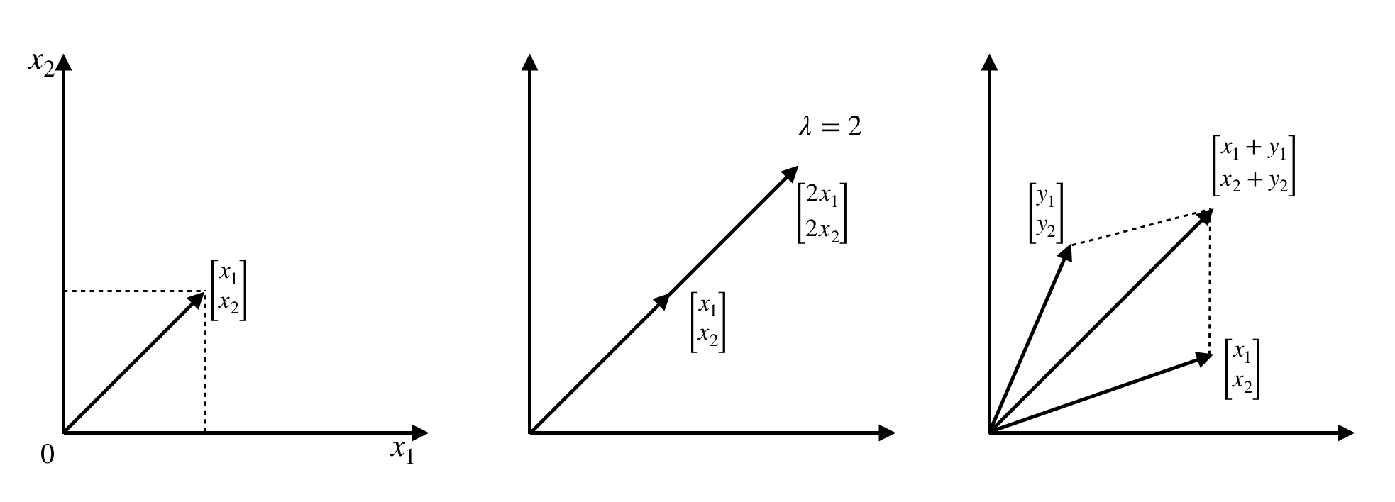
We can, however, multiply scalars with vectors. Let λ be an arbitrary scalar, which we will multiply with the vector  , so that the following applies:

As we can see, λ gets multiplied by each xi in the vector. The result of this operation is that the vector gets scaled by the value of the scalar.
For example, let  , and
, and  . Then, we have the following:

While this works fine for multiplying by a whole number, it doesn't help when working with fractions, but you should be able to guess how it works. Let's see an example.
Let  , and
, and  . Then, we have the following:

There is a very special vector that we can get by multiplying any vector by the scalar, 0. We denote this as 0 and call it the zero vector (a vector containing only zeros).
Linear equations
Linear algebra, at its core, is about solving a set of linear equations, referred to as a system of equations. A large number of problems can be formulated as a system of linear equations.
We have two equations and two unknowns, as follows:

Both equations produce straight lines. The solution to both these equations is the point where both lines meet. In this case, the answer is the point (3, 1).
But for our purposes, in linear algebra, we write the preceding equations as a vector equation that looks like this:

Here, b is the result vector.
Placing the point (3, 1) into the vector equation, we get the following:

As we can see, the left-hand side is equal to the right-hand side, so it is, in fact, a solution! However, I personally prefer to write this as a coefficient matrix, like so:

Using the coefficient matrix, we can express the system of equations as a matrix problem in the form  , where the column vector v is the variable vector. We write this as shown:
 .
.
Going forward, we will express all our problems in this format.
To develop a better understanding, we'll break down the multiplication of matrix A and vector v. It is easiest to think of it as a linear combination of vectors. Let's take a look at the following example with a 3x3 matrix and a 3x1 vector:

It is important to note that matrix and vector multiplication is only possible when the number of columns in the matrix is equal to the number of rows (elements) in the vector.
For example, let's look at the following matrix:

This can be multiplied since the number of columns in the matrix is equal to the number of rows in the vector, but the following matrix cannot be multiplied as the number of columns and number of rows are not equal:

Let's visualize some of the operations on vectors to create an intuition of how they work. Have a look at the following screenshot:
The preceding vectors we dealt with are all in  (in 2-dimensional space), and all resulting combinations of these vectors will also be in
  . The same applies for vectors in
  ,
,  , and
, and  .
.
There is another very important vector operation called the dot product, which is a type of multiplication. Let's take two arbitrary vectors in  , v and w, and find its dot product, like this:

The following is the product:
 .
.
Let's continue, using the same vectors we dealt with before, as follows:

And by taking their dot product, we get zero, which tells us that the two vectors are perpendicular (there is a 90° angle between them), as shown here:

The most common example of a perpendicular vector is seen with the vectors that represent the x axis, the y axis, and so on. In  , we write the x axis vector as
  and the y axis vector as
  . If we take the dot product i•j, we find that it is equal to zero, and they are thus perpendicular.
By combining i and j into a 2x2 matrix, we get the following identity matrix, which is a very important matrix:

The following are some of the scenarios we will face when solving linear equations of the type :
- Let's consider the matrix
 and the equations
  and
and  . If we do the algebra and multiply the first equation by 3, we get
  . But the second equation is equal to zero, which means that these two equations do not intersect and therefore have no solution. When one column is dependent on another—that is, is a multiple of another column—all combinations of
  and
and  lie in the same direction. However, seeing as
  is not a combination of the two aforementioned column vectors and does not lie on the same line, it cannot be a solution to the equation.
 - Let's take the same matrix as before, but this time,
 . Since b is on the line and is a combination of the dependent vectors, there is an infinite number of solutions. We say that b is in the column space of A. While there is only one specific combination of v that produces b, there are infinite combinations of the column vectors that result in the zero vector (0). For example, for any value, a, we have the following:

This leads us to another very important concept, known as the complete solution. The complete solution is all the possible ways to produce  . We write this as
  , where
  .
.
Solving linear equations in n-dimensions
Now that we've dealt with linear equations in 2-dimensions and have developed an understanding of them, let's go a step further and look at equations in 3-dimensions.
Earlier, our equations produced curves in the 2-dimensional space (xy-plane). Now, the equations we will be dealing with will produce planes in 3-dimensional space (xyz-plane).
Let's take an arbitrary 3x3 matrix, as follows:

We know from earlier in having dealt with linear equations in two dimensions that our solution b, as before, is a linear combination of the three column vectors, so that  .
.
The equation  (equation 1) produces a plane, as do
  (equation 2), and
  (equation 3).
When two planes intersect, they intersect at a line; however, when three planes intersect, they intersect at a point. That point is the vector  , which is the solution to our problem.
However, if the three planes do not intersect at a point, there is no solution to the linear equation. This same concept of solving linear equations can be extended to many more dimensions.
Suppose now that we have a system with 15 linear equations and 15 unknown variables. We can use the preceding method and, according to it, we need to find the point that satisfies all the 15 equations—that is, where they intersect (if it exists).
It will look like this:

As you can tell, that's a lot of equations we have to deal with, and the greater the number of dimensions, the harder this becomes to solve.
Solving linear equations using elimination
One of the best ways to solve linear equations is by a systematic method known as elimination. This is a method that allows us to systematically eliminate variables and use substitution to solve equations.
Let's take a look at two equations with two variables, as follows:

After elimination, this becomes the following:

As we can see, the x variable is no longer in the second equation. We can plug the y value back into the first equation and solve for x. Doing this, we find that x = 3 and y = 1.
We call this triangular factorization. There are two types—lower triangular and upper triangular. We solve the upper triangular system from top to bottom using a process known as back substitution, and this works for systems of any size.
Let's solve three equations with three variables, as follows:

We will use upper triangular factorization and eliminate variables, starting with y and then z. Let's start by putting this into our matrix form, as follows:

For our purposes and to make things simpler, we will drop v, the column vector, and get the following result:

Then, exchange row 2 and row 3 with each other, like this:

Then, add row 2 and row 1 together to eliminate the first value in row 2, like this:

Next, multiply row 1 by 3/2 and subtract it from row 3, like this:

Finally, multiply row 2 by 6 and subtract it from row 3, like this:

As you can notice, the values in the matrix now form a triangle pointing upward, which is why we call it upper triangular. By substituting the values back into the previous equation backward (from bottom to top), we can solve, and find that  ,
,  , and
, and  .
.
In summary,  becomes
  , as illustrated here:

To check that our found solution is right, we solve  , using our found values for x, y, and z, like this:

This then becomes the following equation:

And as we can see, the left-hand side is equal to the right-hand side.
After upper triangular factorization, an arbitrary 4x4 matrix will look like this:

We could take this a step further and factorize the upper triangular matrix until we end up with a matrix that contains only the pivot values along the diagonal, and zeros everywhere else. This resulting matrix P essentially fully solves the problem for us without us having to resort to forward or backward substitution, and it looks like this:

But as you can tell, there are a lot of steps involved in getting us from A to P.
There is one other very important factorization method called lower-upper (LU) decomposition. The way it works is we factorize A into an upper triangular matrix U, and record the steps of Gaussian elimination in a lower triangular matrix L, such that  .
.
Let's revisit the matrix we upper-triangular factorized before and put it into LU factorized form, like this:

If we multiply the two matrices on the right, we will get the original matrix A. But how did we get here? Let's go through the steps, as follows:
- We start with
 , so that the following applies:

- We add -1 to what was the identity matrix at l2,1 to represent the operation (row 2)-(-1)(row 1), so it becomes the following:

- We then add
 to the matrix at l3,1 to represent the
  operation, so it becomes the following:

- We then add 6 to the matrix at l3,2 to represent the operation (row 3)-6(row 2), so it becomes the following:

This is the LU factorized matrix we saw earlier.
You might now be wondering what this has to do with solving  , which is very valid. The elimination process tends to work quite well, but we have to additionally apply all the operations we did on A to b as well, and this involves extra steps. However, LU factorization is only applied to A.
Let's now take a look at how we can solve our system of linear equations using this method.
For simplicity, we drop the variables vector and write A and b as follows:
But even this can get cumbersome to write as we go, so we will instead write it in the following way for further simplicity:

We then multiply both sides by  and get the following result:

This tells us that  , and we already know from the preceding equation that
  (so
(so  ). And by using back substitution, we can find the vector v.
In the preceding example, you may have noticed some new notation that I have not yet introduced, but not to worry—we will observe all the necessary notation and operations in the next section.
Matrix operations
Now that we understand how to solve systems of linear equations of the type  where we multiplied a matrix with a column vector, let's move on to dealing with the types of operations we can do with one or more matrices.
Adding matrices
As with scalars and vectors, sometimes we may have to add two or more matrices together, and the process of doing so is rather straightforward. Let's take two  matrices, A and B, and add them:

It is important to note that we can only add matrices that have the same dimensions, and, as you have probably noticed, we add the matrices element-wise.
Multiplying matrices
So far, we have only multiplied a matrix by a column vector. But now, we will multiply a matrix A with another matrix B.
There are four simple rules that will help us in multiplying matrices, listed here:
- Firstly, we can only multiply two matrices when the number of columns in matrix A is equal to the number of rows in matrix B.
- Secondly, the first row of matrix A multiplied by the first column of matrix B gives us the first element in the matrix AB, and so on.
- Thirdly, when multiplying, order matters—specifically, AB ≠ BA.
- Lastly, the element at row i, column j is the product of the ith row of matrix A and the jth column of matrix B.
Let's multiply an arbitrary 4x5 matrix with an arbitrary 5x6 matrix, as follows:

This results in a 4x6 matrix, like this:

From that, we can deduce that in general, the following applies:

Let's take the following two matrices and multiply them, like this:
 and
and 
This will give us the following matrix:
 .
.
The identity matrix has two unique properties in matrix multiplication. When multiplied by any matrix, it returns the original matrix unchanged, and the order of multiplication does not matter—so, AI = IA = A.
For example, let's use the same matrix A from earlier, and multiply it by another matrix B, as follows:

Another very special matrix is the inverse matrix, which is written as A-1. And when we multiply A with A-1, we receive I, the identity matrix.
As mentioned before, the order in which we multiply matters. We must keep the matrices in order, but we do have some flexibility. As we can see in the following equation, the parentheses can be moved:

This is the first law of matrix operations, known as associativity.
The following are three important laws that cannot be broken:
- commutativity:

- distributivity:
 or
or 
- associativity:

As proof that AB ≠ BA, let's take a look at the following example:

This conclusively shows that the two results are not the same.
We know that we can raise numbers to powers, but we can also raise matrices to powers.
If we raise the matrix A to power p, we get the following:
 (multiplying the matrix by itself p times)
There are two additional power laws for matrices— and
and  .
.
Inverse matrices
Let's revisit the concept of inverse matrices and go a little more in depth with them. We know from earlier that AA-1 = I, but not every matrix has an inverse.
There are, again, some rules we must follow when it comes to finding the inverses of matrices, as follows:
- The inverse only exists if, through the process of upper or lower triangular factorization, we obtain all the pivot values on the diagonal.
- If the matrix is invertible, it has only one unique inverse matrix—that is, if AB = I and AC = I, then B = C.
- If A is invertible, then to solve Av = b we multiply both sides by A-1 and get AA-1v = A-1b, which finally gives us = A-1b.
- If v is nonzero and b = 0, then the matrix does not have an inverse.
- 2 x 2 matrices are invertible only if ad - bc ≠ 0, where the following applies:

And ad - bc is called the determinant of A. A-1 involves dividing each element in the matrix by the determinant.
- Lastly, if the matrix has any zero values along the diagonal, it is non-invertible.
Sometimes, we may have to invert the product of two matrices, but that is only possible when both the matrices are individually invertible (follow the rules outlined previously).
For example, let's take two matrices A and B, which are both invertible. Then,  so that
  .
.
Matrix transpose
Let's take an  matrix A. If the matrix's transpose is B, then the dimensions of B are
  , such that:
  . Here is the matrix A:

Then, the matrix B is as given:
 .
.
Essentially, we can think of this as writing the columns of A as the rows of the transposed matrix, B.
A symmetric matrix is a special kind of matrix. It is an n×n matrix that, when transposed, is exactly the same as before we transposed it.
The following are the properties of inverses and transposes:


If A is an invertible matrix, then so is AT, and so (A-1)T = (AT)-1 = A-T.
Permutations
In the example on solving systems of linear equations, we swapped the positions of rows 2 and 3. This is known as a permutation.
When we are doing triangular factorization, we want our pivot values to be along the diagonal of the matrix, but this won't happen every time—in fact, it usually won't. So, instead, what we do is swap the rows so that we get our pivot values where we want them.
But that is not their only use case. We can also use them to scale individual rows by a scalar value or add rows to or subtract rows from other rows.
Let's start with some of the more basic permutation matrices that we obtain by swapping the rows of the identity matrix. In general, we have n! possible permutation matrices that can be formed from an nxn identity matrix. In this example, we will use a 3×3 matrix and therefore have six permutation matrices, and they are as follows:
 This matrix makes no change to the matrix it is applied on.
 This matrix swaps rows two and three of the matrix it is applied on.
 This matrix swaps rows one and two of the matrix it is applied on.
 This matrix shifts rows two and three up one and moves row one to the position of row three of the matrix it is applied on.
 This matrix shifts rows one and two down one and moves row three to the row-one position of the matrix it is applied on.
 This matrix swaps rows one and three of the matrix it is applied on.
It is important to note that there is a particularly fascinating property of permutation matrices that states that if we have a matrix  and it is invertible, then there exists a permutation matrix that when applied to A will give us the LU factor of A. We can express this like so:

Vector spaces and subspaces
In this section, we will explore the concepts of vector spaces and subspaces. These are very important to our understanding of linear algebra. In fact, if we do not have an understanding of vector spaces and subspaces, we do not truly have an understanding of how to solve linear algebra problems.
Spaces
Vector spaces are one of the fundamental settings for linear algebra, and, as the name suggests, they are spaces where all vectors reside. We will denote the vector space with V.
The easiest way to think of dimensions is to count the number of elements in the column vector. Suppose we have  , then
  .
.  is a straight line,
  is all the possible points in the xy-plane, and
  is all the possible points in the xyz-plane—that is, 3-dimensional space, and so on.
The following are some of the rules for vector spaces:
- There exists in V an additive identity element such that
 for all
  .
. - For all
 , there exists an additive inverse such that
  .
. - For all
 , there exists a multiplicative identity such that
  .
. - Vectors are commutative, such that for all
 ,
,  .
. - Vectors are associative, such that
 .
. - Vectors have distributivity, such that
 and
and  for all
  and for all
  .
.
A set of vectors is said to be linearly independent if  , which implies that
  .
.
Another important concept for us to know is called span. The span of  is the set of all linear combinations that can be made using the n vectors. Therefore,
  if the vectors are linearly independent and span V completely; then, the vectors
  are the basis of V.
Therefore, the dimension of V is the number of basis vectors we have, and we denote it dimV.
Subspaces
Subspaces are another very important concept that state that we can have one or many vector spaces inside another vector space. Let's suppose V is a vector space, and we have a subspace  . Then, S can only be a subspace if it follows the three rules, stated as follows:

 and
and  , which implies that S is closed under addition
 and
and  so that
  , which implies that S is closed under scalar multiplication
If  , then their sum is
  , where the result is also a subspace of V.
The dimension of the sum  is as follows:

Linear maps
A linear map is a function  , where V and W are both vector spaces. They must satisfy the following criteria:
 , for all
 , for all
  and
and 
Linear maps tend to preserve the properties of vector spaces under addition and scalar multiplication. A linear map is called a homomorphism of vector spaces; however, if the homomorphism is invertible (where the inverse is a homomorphism), then we call the mapping an isomorphism.
When V and W are isomorphic, we denote this as  , and they both have the same algebraic structure.
If V and W are vector spaces in  , and
, and  , then it is called a natural isomorphism. We write this as follows:

Here,  and
and  are the bases of V and W. Using the preceding equation, we can see that
  , which tells us that
  is an isomorphism.
Let's take the same vector spaces V and W as before, with bases and  respectively. We know that is a linear map, and the matrix T that has entries Aij, where
  and
and  can be defined as follows:
 .
.
From our knowledge of matrices, we should know that the jth column of A contains Tvj in the basis of W.
Thus,  produces a linear map
  , which we write as
  .
.
Image and kernel
When dealing with linear mappings, we will often encounter two important terms: the image and the kernel, both of which are vector subspaces with rather important properties.
The kernel (sometimes called the null space) is 0 (the zero vector) and is produced by a linear map, as follows:

And the image (sometimes called the range) of T is defined as follows:
 such that
  .
.
V and W are also sometimes known as the domain and codomain of T.
It is best to think of the kernel as a linear mapping that maps the vectors  to
to  . The image, however, is the set of all possible linear combinations of
  that can be mapped to the set of vectors
  .
.
The Rank-Nullity theorem (sometimes referred to as the fundamental theorem of linear mappings) states that given two vector spaces V and W and a linear mapping  , the following will remain true:
 .
.
Metric space and normed space
Metrics help define the concept of distance in Euclidean space (denoted by  ). Metric spaces, however, needn't always be vector spaces. We use them because they allow us to define limits for objects besides real numbers.
So far, we have been dealing with vectors, but what we don't yet know is how to calculate the length of a vector or the distance between two or more vectors, as well as the angle between two vectors, and thus the concept of orthogonality (perpendicularity). This is where Euclidean spaces come in handy. In fact, they are the fundamental space of geometry. This may seem rather trivial at the moment, but their importance will become more apparent to you as we get further on in the book.
In Euclidean space, we tend to refer to vectors as points.
A metric on a set S is defined as a function  and satisfies the following criteria:
 , and when
  then
then 

 (known as the triangle inequality)
For all  .
.
That's all well and good, but how exactly do we calculate distance?
Let's suppose we have two points,  and
and  ; then, the distance between them can be calculated as follows:

And we can extend this to find the distance of points in  , as follows:

While metrics help with the notion of distance, norms define the concept of length in Euclidean space.
A norm on a vector space is a function  , and satisfies the following conditions:
 , and when
  then
then 

 (also known as the triangle inequality)
For all  and
and  .
.
It is important to note that any norm on the vector space creates a distance metric on the said vector space, as follows:

This satisfies the rules for metrics, telling us that a normed space is also a metric space.
In general, for our purposes, we will only be concerned with four norms on  , as follows:


 (this applies only if
  )
)
If you look carefully at the four norms, you can notice that the 1- and 2-norms are versions of the p-norm. The  -norm, however, is a limit of the p-norm, as p tends to infinity.
Using these definitions, we can define two vectors to be orthogonal if the following applies:

Inner product space
An inner product on a vector space is a function  , and satisfies the following rules:

 and
and 

For all  and
and  .
.
It is important to note that any inner product on the vector space creates a norm on the said vector space, which we see as follows:

We can notice from these rules and definitions that all inner product spaces are also normed spaces, and therefore also metric spaces.
Another very important concept is orthogonality, which in a nutshell means that two vectors are perpendicular to each other (that is, they are at a right angle to each other) from Euclidean space.
Two vectors are orthogonal if their inner product is zero—that is,  . As a shorthand for perpendicularity, we write
  .
.
Additionally, if the two orthogonal vectors are of unit length—that is,  , then they are called orthonormal.
In general, the inner product in  is as follows:

Matrix decompositions
Matrix decompositions are a set of methods that we use to describe matrices using more interpretable matrices and give us insight to the matrices' properties.
Determinant
Earlier, we got a quick glimpse of the determinant of a square 2x2 matrix when we wanted to determine whether a square matrix was invertible. The determinant is a very important concept in linear algebra and is used frequently in the solving of systems of linear equations.
Notationally, the determinant is usually written as either  or
or  .
.
Let's take an arbitrary n×n matrix A, as follows:

We will also take its determinant, as follows:

The determinant reduces the matrix to a real number (or, in other words, maps A onto a real number).
We start by checking if a square matrix is invertible. Let's take a 2x2 matrix, and from the earlier definition, we know that the matrix applied to its inverse produces the identity matrix. It works no differently than when we multiply a with  (only true when
  ), which produces 1, except with matrices. Therefore, AA-1 = I.
Let's go ahead and find the inverse of our matrix, as follows:

A is invertible only when  , and this resulting value is what we call the determinator.
Now that we know how to find the determinant in the 2x2 case, let's move on to a 3x3 matrix and find its determinant. It looks like this:

This produces the following:

I know that probably looks more intimidating, but it's really not. Take a moment to look carefully at what we did and how this would work for a larger n×n matrix.
If we have an n×n matrix and if it can be triangularly factorized (upper or lower), then its determinant will be the product of all the pivot values. For the sake of simplicity, we will represent all triangularly factorizable matrices with T. Therefore, the determinant can be written like so:

Looking at the preceding 3×3 matrix example, I'm sure you've figured out that computing the determinant for matrices where n > 3 is quite a lengthy process. Luckily, there is a way in which we can simplify the calculation, and this is where the Laplace expansion comes to the rescue.
When we want to find the determinant of an n×n matrix, the Laplace expansion finds the determinant of (n×1)×(n×1) matrices and does so repeatedly until we get to 2×2 matrices. In general, we can calculate the determinant of an n×n matrix using 2×2 matrices.
Let's again take an n-dimensional square matrix, where  . We then expand for all
  , as follows:
- Expansion along row i:

- Expansion along row j:

And  is a sub-matrix of
  , which we get after removing row i and column j.
For example, we have a 3×3 matrix, as follows:

We want to find its determinant using the Laplace expansion along the first row. This results in the following:

We can now use the preceding equation from the 2×2 case and calculate the determinant for A, as follows:
 .
.
Here are some of the very important properties of determinants that are important to know:


There is one other additional property of the determinant, and it is that we can use it to find the volume of an object in  whose vertices are formed by the column vectors in the matrix.
As an example, let's take a parallelogram in  with the vectors
  and
and  . By taking the determinant of the 2×2 matrix, we find the area of the shape (we can only find the volume for objects in
  or higher), as follows:

You are welcome to try it for any 3×3 matrix for yourselves as practice.
Eigenvalues and eigenvectors
Let's imagine an arbitrary real n×n matrix, A. It is very possible that when we apply this matrix to some vector, they are scaled by a constant value. If this is the case, we say that the nonzero  -dimensional vector is an eigenvector of A, and it corresponds to an eigenvalue λ. We write this as follows:

Let's consider again a matrix A that has an eigenvector x and a corresponding eigenvalue λ. Then, the following rules will apply:
- If we have a matrix A and it has been shifted from its current position to
 , then it has the eigenvector x and the corresponding eigenvalue
  , for all
  , so that
  .
. - If the matrix A is invertible, then x is also an eigenvector of the inverse of the matrix,
 , with the corresponding eigenvalue
  .
.  for any
  .
.
We know from earlier in the chapter that whenever we multiply a matrix and a vector, the direction of the vector is changed, but this is not the case with eigenvectors. They are in the same direction as A, and thus x remains unchanged. The eigenvalue, being a scalar value, tells us whether the eigenvector is being scaled, and if so, how much, as well as if the direction of the vector has changed.
Another very fascinating property the determinant has is that it is equivalent to the product of the eigenvalues of the matrix, and it is written as follows:

But this isn't the only relation that the determinant has with eigenvalues. We can rewrite in the form . And since this is equal to zero, this means it is a non-invertible matrix, and therefore its determinant too must be equal to zero. Using this, we can use the determinant to find the eigenvalues. Let's see how.
Suppose we have  . Then, its determinant is shown as follows:

We can rewrite this as the following quadratic equation:

We know that the quadratic equation will give us both the eigenvalues  . So, we plug our values into the quadratic formula and get our roots.
Another interesting property is that when we have triangular matrices such as the ones we found earlier in this chapter, their eigenvalues are the pivot values. So, if we want to find the determinant of a triangular matrix, then all we have to do is find the product of all the entries along the diagonal.
Trace
Given an n×n matrix A, the sum of all the entries on the diagonal is called the trace. We write it like so:

The following are four important properties of the trace:


A very interesting property of the trace is that it is equal to the sum of its eigenvalues, so that the following applies:

Orthogonal matrices
The concept of orthogonality arises frequently in linear algebra. It's really just a fancy word for perpendicularity, except it goes beyond two dimensions or a pair of vectors.
But to get an understanding, let's start with two column vectors  . If they are orthogonal, then the following holds:
 .
.
Orthogonal matrices are a special kind of matrix where the columns are pairwise orthonormal. What this means is that we have a matrix  with the following property:

Then, we can deduce that  (that is, the transpose of Q is also the inverse of Q).
As with other types of matrices, orthogonal matrices have some special properties.
Firstly, they preserve inner products, so that the following applies:
 .
.
This brings us to the second property, which states that 2-norms are preserved for orthogonal matrices, which we see as follows:

When multiplying by orthogonal matrices, you can think of it as a transformation that preserves length, but the vector may be rotated about the origin by some degree.
The most well-known orthogonal matrix that is also orthonormal is a special matrix we have dealt with a few times already. It is the identity matrix I, and since it represents a unit of length in the direction of axes, we generally refer to it as the standard basis.
Diagonalization and symmetric matrices
Let's suppose we have a matrix  that has
  eigenvectors. We put these vectors into a matrix X that is invertible and multiply the two matrices. This gives us the following:

We know from  that when dealing with matrices, this becomes
  , where
  and each xi has a unique λi. Therefore,
  .
.
Let's move on to symmetric matrices. These are special matrices that, when transposed, are the same as the original, implying that  and for all
  ,
,  . This may seem rather trivial, but its implications are rather strong.
The spectral theorem states that if a matrix is a symmetric matrix, then there exists an orthonormal basis for  , which contains the eigenvectors of A.
This theorem is important to us because it allows us to factorize symmetric matrices. We call this spectral decomposition (also sometimes referred to as Eigendecomposition).
Suppose we have an orthogonal matrix Q, with the orthonormal basis of eigenvectors  and being the matrix with corresponding eigenvalues.
From earlier, we know that  for all
  ; therefore, we have the following:

 s need to multiply the individual columns of Q.
By multiplying both sides by QT, we get the following result:

Singular value decomposition
Singular Value Decomposition (SVD) is widely used in linear algebra and is known for its strength, particularly arising from the fact that every matrix has an SVD. It looks like this:

For our purposes, let's suppose  ,
,  ,
,  , and
, and  , and that U, V are orthogonal matrices, whereas ∑ is a matrix that contains singular values (denoted by σi) of A along the diagonal.
∑ in the preceding equation looks like this:

We can also write the SVD like so:

Here, ui, vi are the column vectors of U, V.
Cholesky decomposition
As I'm sure you've figured out by now, there is more than one way to factorize a matrix, and there are special methods for special matrices.
The Cholesky decomposition is square root-like and works only on symmetric positive definite matrices.
This works by factorizing A into the form LLT. Here, L, as before, is a lower triangular matrix.
Do develop some intuition. It looks like this:

However, here, L is called a Cholesky factor.
Let's take a look at the case where  .
.
We know from the preceding matrix that  ; therefore, we have the following:

Let's multiply the upper and lower triangular matrices on the right, as follows:

Writing out A fully and equating it to our preceding matrix gives us the following:

We can then compare, element-wise, the corresponding entries of A and LLT and solve algebraically for  , as follows:

We can repeat this process for any symmetric positive definite matrix, and compute the li,j values given ai,j.
Summary
With this, we conclude our chapter on linear algebra. So far, we have learned all the fundamental concepts of linear algebra, such as matrix multiplication and factorization, that will lead you on your way to gaining a deep understanding of how deep neural networks (DNNs) work and are designed, and what it is that makes them so powerful.
In the next chapter, we will be learning about calculus and will combine it with the concepts learned earlier on in this chapter to understand vector calculus.