Home Data Modern Computer Vision with PyTorch

Modern Computer Vision with PyTorch

By V Kishore Ayyadevara , Yeshwanth Reddy
ai-assist-svg-icon Book + AI Assistant
eBook + AI Assistant $45.99 $31.99
Print $65.99
Subscription $15.99 $10 p/m for three months
ai-assist-svg-icon NEW: AI Assistant (beta) Available with eBook, Print, and Subscription.
ai-assist-svg-icon NEW: AI Assistant (beta) Available with eBook, Print, and Subscription. $10 p/m for first 3 months. $15.99 p/m after that. Cancel Anytime! ai-assist-svg-icon NEW: AI Assistant (beta) Available with eBook, Print, and Subscription.
What do you get with a Packt Subscription?
Gain access to our AI Assistant (beta) for an exclusive selection of 500 books, available during your subscription period. Enjoy a personalized, interactive, and narrative experience to engage with the book content on a deeper level.
This book & 7000+ ebooks & video courses on 1000+ technologies
60+ curated reading lists for various learning paths
50+ new titles added every month on new and emerging tech
Early Access to eBooks as they are being written
Personalised content suggestions
Customised display settings for better reading experience
50+ new titles added every month on new and emerging tech
Playlists, Notes and Bookmarks to easily manage your learning
Mobile App with offline access
What do you get with a Packt Subscription?
This book & 6500+ ebooks & video courses on 1000+ technologies
60+ curated reading lists for various learning paths
50+ new titles added every month on new and emerging tech
Early Access to eBooks as they are being written
Personalised content suggestions
Customised display settings for better reading experience
50+ new titles added every month on new and emerging tech
Playlists, Notes and Bookmarks to easily manage your learning
Mobile App with offline access
What do you get with eBook + Subscription?
Download this book in EPUB and PDF formats, plus a monthly download credit
This book & 6500+ ebooks & video courses on 1000+ technologies
60+ curated reading lists for various learning paths
50+ new titles added every month on new and emerging tech
Early Access to eBooks as they are being written
Personalised content suggestions
Customised display settings for better reading experience
50+ new titles added every month on new and emerging tech
Playlists, Notes and Bookmarks to easily manage your learning
Mobile App with offline access
What do you get with a Packt Subscription?
Gain access to our AI Assistant (beta) for an exclusive selection of 500 books, available during your subscription period. Enjoy a personalized, interactive, and narrative experience to engage with the book content on a deeper level.
This book & 6500+ ebooks & video courses on 1000+ technologies
60+ curated reading lists for various learning paths
50+ new titles added every month on new and emerging tech
Early Access to eBooks as they are being written
Personalised content suggestions
Customised display settings for better reading experience
50+ new titles added every month on new and emerging tech
Playlists, Notes and Bookmarks to easily manage your learning
Mobile App with offline access
What do you get with eBook?
Along with your eBook purchase, enjoy AI Assistant (beta) access in our online reader for a personalized, interactive reading experience.
Download this book in EPUB and PDF formats
Access this title in our online reader
DRM FREE - Read whenever, wherever and however you want
Online reader with customised display settings for better reading experience
What do you get with video?
Download this video in MP4 format
Access this title in our online reader
DRM FREE - Watch whenever, wherever and however you want
Online reader with customised display settings for better learning experience
What do you get with video?
Stream this video
Access this title in our online reader
DRM FREE - Watch whenever, wherever and however you want
Online reader with customised display settings for better learning experience
What do you get with Audiobook?
Download a zip folder consisting of audio files (in MP3 Format) along with supplementary PDF
What do you get with Exam Trainer?
Flashcards, Mock exams, Exam Tips, Practice Questions
Access these resources with our interactive certification platform
Mobile compatible-Practice whenever, wherever, however you want
ai-assist-svg-icon NEW: AI Assistant (beta) Available with eBook, Print, and Subscription. ai-assist-svg-icon NEW: AI Assistant (beta) Available with eBook, Print, and Subscription. BUY NOW $10 p/m for first 3 months. $15.99 p/m after that. Cancel Anytime! ai-assist-svg-icon NEW: AI Assistant (beta) Available with eBook, Print, and Subscription.
eBook + AI Assistant $45.99 $31.99
Print $65.99
Subscription $15.99 $10 p/m for three months
What do you get with a Packt Subscription?
Gain access to our AI Assistant (beta) for an exclusive selection of 500 books, available during your subscription period. Enjoy a personalized, interactive, and narrative experience to engage with the book content on a deeper level.
This book & 7000+ ebooks & video courses on 1000+ technologies
60+ curated reading lists for various learning paths
50+ new titles added every month on new and emerging tech
Early Access to eBooks as they are being written
Personalised content suggestions
Customised display settings for better reading experience
50+ new titles added every month on new and emerging tech
Playlists, Notes and Bookmarks to easily manage your learning
Mobile App with offline access
What do you get with a Packt Subscription?
This book & 6500+ ebooks & video courses on 1000+ technologies
60+ curated reading lists for various learning paths
50+ new titles added every month on new and emerging tech
Early Access to eBooks as they are being written
Personalised content suggestions
Customised display settings for better reading experience
50+ new titles added every month on new and emerging tech
Playlists, Notes and Bookmarks to easily manage your learning
Mobile App with offline access
What do you get with eBook + Subscription?
Download this book in EPUB and PDF formats, plus a monthly download credit
This book & 6500+ ebooks & video courses on 1000+ technologies
60+ curated reading lists for various learning paths
50+ new titles added every month on new and emerging tech
Early Access to eBooks as they are being written
Personalised content suggestions
Customised display settings for better reading experience
50+ new titles added every month on new and emerging tech
Playlists, Notes and Bookmarks to easily manage your learning
Mobile App with offline access
What do you get with a Packt Subscription?
Gain access to our AI Assistant (beta) for an exclusive selection of 500 books, available during your subscription period. Enjoy a personalized, interactive, and narrative experience to engage with the book content on a deeper level.
This book & 6500+ ebooks & video courses on 1000+ technologies
60+ curated reading lists for various learning paths
50+ new titles added every month on new and emerging tech
Early Access to eBooks as they are being written
Personalised content suggestions
Customised display settings for better reading experience
50+ new titles added every month on new and emerging tech
Playlists, Notes and Bookmarks to easily manage your learning
Mobile App with offline access
What do you get with eBook?
Along with your eBook purchase, enjoy AI Assistant (beta) access in our online reader for a personalized, interactive reading experience.
Download this book in EPUB and PDF formats
Access this title in our online reader
DRM FREE - Read whenever, wherever and however you want
Online reader with customised display settings for better reading experience
What do you get with video?
Download this video in MP4 format
Access this title in our online reader
DRM FREE - Watch whenever, wherever and however you want
Online reader with customised display settings for better learning experience
What do you get with video?
Stream this video
Access this title in our online reader
DRM FREE - Watch whenever, wherever and however you want
Online reader with customised display settings for better learning experience
What do you get with Audiobook?
Download a zip folder consisting of audio files (in MP3 Format) along with supplementary PDF
What do you get with Exam Trainer?
Flashcards, Mock exams, Exam Tips, Practice Questions
Access these resources with our interactive certification platform
Mobile compatible-Practice whenever, wherever, however you want
  1. Free Chapter
    Artificial Neural Network Fundamentals
About this book
Deep learning is the driving force behind many recent advances in various computer vision (CV) applications. This book takes a hands-on approach to help you to solve over 50 CV problems using PyTorch1.x on real-world datasets. You’ll start by building a neural network (NN) from scratch using NumPy and PyTorch and discover best practices for tweaking its hyperparameters. You’ll then perform image classification using convolutional neural networks and transfer learning and understand how they work. As you progress, you’ll implement multiple use cases of 2D and 3D multi-object detection, segmentation, human-pose-estimation by learning about the R-CNN family, SSD, YOLO, U-Net architectures, and the Detectron2 platform. The book will also guide you in performing facial expression swapping, generating new faces, and manipulating facial expressions as you explore autoencoders and modern generative adversarial networks. You’ll learn how to combine CV with NLP techniques, such as LSTM and transformer, and RL techniques, such as Deep Q-learning, to implement OCR, image captioning, object detection, and a self-driving car agent. Finally, you'll move your NN model to production on the AWS Cloud. By the end of this book, you’ll be able to leverage modern NN architectures to solve over 50 real-world CV problems confidently.
Publication date:
November 2020
Publisher
Packt
Pages
824
ISBN
9781839213472

 
Artificial Neural Network Fundamentals

An Artificial Neural Network (ANN) is a supervised learning algorithm that is loosely inspired by the way the human brain functions. Similar to the way neurons are connected and activated in the human brain, a neural network takes input and passes it through a function, resulting in certain subsequent neurons getting activated, and consequently producing the output.

There are several standard ANN architectures. The universal approximation theorem says that we can always find a large enough neural network architecture with the right set of weights that can exactly predict any output for any given input. This means, for a given dataset/task we can create an architecture and keep adjusting its weights until the ANN predicts what we want it to predict. Adjusting the weights until this happens is called training the neural network. Successful training on large datasets and customized architecture is how ANNs have gained prominence in solving various relevant tasks.

One of the prominent tasks in computer vision is to recognize the class of the object present in an image. ImageNet was a competition held to identify the class of objects present in an image. The reduction in classification error rate over the years is as follows:

The year 2012 was when a neural network (AlexNet) was used in the winning solution of the competition. As you can see from the preceding chart, there was a considerable reduction in errors from the year 2011 to the year 2012 by leveraging neural networks. Over time since then, with more deep and complex neural networks, the classification error kept reducing and has beaten human-level performance. This gives a solid motivation for us to learn and implement neural networks for our custom tasks, where applicable.

In this chapter, we will create a very simple architecture on a simple dataset and mainly focus on how the various building blocks (feedforward, backpropagation, learning rate) of an ANN help in adjusting the weights so that the network learns to predict the expected outputs from given inputs. We will first learn, mathematically, what a neural network is, and then build one from scratch to have a solid foundation. Then we will learn about each component responsible for training the neural network and code them as well. Overall, we will cover the following topics:

  • Comparing AI and traditional machine learning
  • Learning about the artificial neural network building blocks
  • Implementing feedforward propagation
  • Implementing backpropagation
  • Putting feedforward propagation and backpropagation together
  • Understanding the impact of the learning rate
  • Summarizing the training process of a neural network
 

Comparing AI and traditional machine learning

Traditionally, systems were made intelligent by using sophisticated algorithms written by programmers.

For example, say you are interested in recognizing whether a photo contains a dog or not. In the traditional Machine Learning (ML) setting, an ML practitioner or a subject matter expert first identifies the features that need to be extracted from images. Then they extract those features and pass them through a well-written algorithm that deciphers the given features to tell whether the image is of a dog or not. The following diagram illustrates the same idea:

Take the following samples:

From the preceding images, a simple rule might be that if an image contains three black circles aligned in a triangular shape, it can be classified as a dog. However, this rule would fail against this deceptive close-up of a muffin:

Of course, this rule also fails when shown an image with anything other than a dog's face close up. Naturally, therefore, the number of manual rules we'd need to create for the accurate classification of multiple types can be exponential, especially as images become more complex. Therefore, the traditional approach works well in a very constrained environment (say, taking a passport photo where all the dimensions are constrained within millimeters) and works badly in an unconstrained environment, where every image varies a lot.

We can extend the same line of thought to any domain, such as text or structured data. In the past, if someone was interested in programming to solve a real-world task, it became necessary for them to understand everything about the input data and write as many rules as possible to cover every scenario. This is tedious and there is no guarantee that all new scenarios would follow said rules.

However, by leveraging artificial neural networks, we can do this in a single step.

Neural networks provide the unique benefit of combining feature extraction (hand-tuning) and use those features for classification/regression in a single shot with little manual feature engineering. Both these subtasks only require labeled data (for example, which pictures are dogs and which pictures are not dogs) and neural network architecture. It does not require a human to come up with rules to classify an image, which takes away the majority of the burden traditional techniques impose on the programmer.

Notice that the main requirement is that we provide a considerable amount of examples for the task that needs a solution. For example, in the preceding case, we need to provide lots and lots of dog and not-dog pictures to the model so it learns the features. A high-level view of how neural networks are leveraged for the task of classification is as follows:

Now that we have gained a very high-level overview of the fundamental reason why neural networks perform better than traditional computer vision methods, let's gain a deeper understanding of how neural networks work throughout the various sections in this chapter.


Learning about the artificial neural network building blocks

An ANN is a collection of tensors (weights) and mathematical operations, arranged in such a way to loosely replicate the functioning of a human brain. It can be viewed as a mathematical function that takes in one or more tensors as inputs and predicts one or more tensors as outputs. The arrangement of operations that connects these inputs to outputs is referred to as the architecture of the neural network – which we can customize based on the task at hand, that is, based on whether the problem contains structured (tabular) or unstructured (image, text, audio) data (which is the list of input and output tensors).

An ANN is made up of the following:

  • Input layers: These layers take the independent variables as input.
  • Hidden (intermediate) layers: These layers connect the input and output layers while performing transformations on top of input data. Furthermore, the hidden layers contain nodes (units/circles in the following diagram) to modify their input values into higher-/lower-dimensional values. The functionality to achieve a more complex representation is achieved by using various activation functions that modify the values of the nodes of intermediate layers.
  • Output layer: This contains the values the input variables are expected to result in.

With this in mind, the typical structure of a neural network is as follows:

The number of nodes (circles in the preceding diagram) in the output layer depends on the task at hand and whether we are trying to predict a continuous variable or a categorical variable. If the output is a continuous variable, the output has one node. If the output is categorical with m possible classes, there will be m nodes in the output layer. Let's zoom into one of the nodes/neurons and see what's happening. A neuron transforms its inputs as follows:

In the preceding diagram, x1,x2, ..., xn are the input variables, and w0 is the bias term (similar to the way we have a bias in linear/logistic regression).

Note that w1,w2, ..., wn are the weights given to each of the input variables and w0 is the bias term. The output value a is calculated as follows:

As you can see, it is the sum of the products of weight and input pairs followed by an additional function f (the bias term + sum of products). The function f is the activation function that is used to apply non-linearity on top of this sum of products. More details on the activation functions will be provided in the next section, on feedforward propagation. Further, higher nonlinearity can be achieved by having more than one hidden layer, stacking multitudes of neurons.

At a high level, a neural network is a collection of nodes where each node has an adjustable float value and the nodes are interconnected as a graph to return outputs in a format that is dictated by the architecture of the network. The network constitutes three main parts: the input layer, the hidden layer(s), and the output layer. Note that you can have a higher number (n) of hidden layers, with the term deep learning referring to the greater number of hidden layers. Typically, more hidden layers are needed when the neural network has to comprehend something complicated such as image recognition.

With the architecture of a neural network understood, in the next section, we will learn about feedforward propagation, which helps in estimating the amount of error (loss) the network architecture has.


Implementing feedforward propagation

To build a strong foundational understanding of how feedforward propagation works, we'll go through a toy example of training a neural network where the input to the neural network is (1, 1) and the corresponding (expected) output is 0. Here, we are going to find the optimal weights of the neural network based on this single input-output pair. However, you should note that in reality, there will be thousands of data points on which an ANN is trained.

Our neural network architecture for this example contains one hidden layer with three nodes in it, as follows:

Every arrow in the preceding diagram contains exactly one float value (weight) that is adjustable. There are 9 (6 in the first hidden layer and 3 in the second) floats that we need to find, so that when the input is (1,1), the output is as close to (0) as possible. This is what we mean by training the neural network. We have not introduced a bias value yet, for simplicity purposes only – the underlying logic remains the same.

In the subsequent sections, we will learn the following about the preceding network:

  • Calculating hidden layer values
  • Performing non-linear activations
  • Estimating the output layer value
  • Calculating the loss value corresponding to the expected value

Calculating the hidden layer unit values

We'll now assign weights to all of the connections. In the first step, we assign weights randomly across all the connections. And in general, neural networks are initialized with random weights before the training starts. Again, for simplicity, while introducing the topic, we will not include the bias value while learning about feedforward propagation and backpropagation. But we will have it while implementing both feedforward propagation and backpropagation from scratch.

Let's start with initial weights that are randomly initialized between 0 and 1, but note that the final weights after the training process of a neural network don't need to be between a specific set of values. A formal representation of weights and values in the network is provided in the following diagram (left half) and the randomly initialized weights are provided in the network in the right half.

In the next step, we perform the multiplication of the input with weights to calculate the values of hidden units in the hidden layer.

The hidden layer's unit values before activation are obtained as follows:

The hidden layer's unit values (before activation) that are calculated here are also shown in the following diagram:

Now, we will pass the hidden layer values through a non-linearity activation. Note that, if we do not apply a non-linear activation function in the hidden layer, the neural network becomes a giant linear connection from input to output, no matter how many hidden layers exist.

Applying the activation function

Activation functions help in modeling complex relations between the input and the output.

Some of the frequently used activation functions are calculated as follows (where x is the input):

Visualizations of each of the preceding activations for various input values are as follows:

For our example, let’s use the sigmoid (logistic) function for activation.

By applying sigmoid (logistic) activation, S(x), to the three hidden layer sums, we get the following values after sigmoid activation:

Now that we have obtained the hidden layer values after activation, in the next section, we will obtain the output layer values.

Calculating the output layer values

So far, we have calculated the final hidden layer values after applying the sigmoid activation. Using the hidden layer values after activation, and the weight values (which are randomly initialized in the first iteration), we will calculate the output value for our network:

We perform the sum of products of the hidden layer values and weight values to calculate the output value. Another reminder: we excluded the bias terms that need to be added at each unit(node), only to simplify our understanding of the working details of feedforward propagation and backpropagation for now and will include it while coding up feedforward propagation and backpropagation:

Because we started with a random set of weights, the value of the output node is very different from the target. In this case, the difference is 1.235 (remember, the target is 0). In the next section, we will learn about calculating the loss value associated with the network in its current state.

Calculating loss values

Loss values (alternatively called cost functions) are the values that we optimize for in a neural network. To understand how loss values get calculated, let's look at two scenarios:

  • Categorical variable prediction
  • Continuous variable prediction

Calculating loss during continuous variable prediction

Typically, when the variable is continuous, the loss value is calculated as the mean of the square of the difference in actual values and predictions, that is, we try to minimize the mean squared error by varying the weight values associated with the neural network. The mean squared error value is calculated as follows:

In the preceding equation, is the actual output. is the prediction computed by the neural network (whose weights are stored in the form of ), where its input is , and m is the number of rows in the dataset.

The key takeaway should be the fact that for every unique set of weights, the neural network would predict a different loss and we need to find the golden set of weights for which the loss is zero (or, in realistic scenarios, as close to zero as possible).

In our example, let's assume that the outcome that we are predicting is continuous. In that case, the loss function value is the mean squared error, which is calculated as follows:

Now that we understand how to calculate the loss value for a continuous variable, in the next section, we will learn about calculating the loss value for a categorical variable.

Calculating loss during categorical variable prediction

When the variable to predict is discrete (that is, there are only a few categories in the variable), we typically use a categorical cross-entropy loss function. When the variable to predict has two distinct values within it, the loss function is binary cross-entropy.

Binary cross-entropy is calculated as follows:

y is the actual value of the output, p is the predicted value of the output, and m is the total number of data points.

Categorical cross-entropy is calculated as follows:

y is the actual value of the output, p is the predicted value of the output, m is the total number of data points, and C is the total number of classes.

A simple way of visualizing cross-entropy loss is to look at the prediction matrix itself. Say you are predicting five classes – Dog, Cat, Rat, Cow, and Hen – in an image recognition problem. The neural network would necessarily have five neurons in the last layer with softmax activation (more on softmax in the next section). It will be thus forced to predict a probability for every class, for every data point. Say there are five images and the prediction probabilities look like so (the highlighted cell in each row corresponds to the target class):

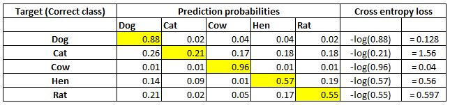
Note that each row sums to 1. In the first row, when the target is Dog and the prediction probability is 0.88, the corresponding loss is 0.128 (which is the negative of the log of 0.88). Similarly, other losses are computed. As you can see, the loss value is less when the probability of the correct class is high. As you know, the probabilities range between 0 and 1. So, the minimum possible loss can be 0 (when the probability is 1) and the maximum loss can be infinity when the probability is 0.

The final loss within a dataset is the mean of all individual losses across all rows.

Now that we have a solid understanding of calculating mean squared error loss and cross-entropy loss, let's get back to our toy example. Assuming our output is a continuous variable, we will learn how to minimize the loss value using backpropagation in a later section. We will update the weight values (which were initialized randomly earlier) to minimize the loss (). But, before that, let's first code feedforward propagation in Python using NumPy arrays to solidify our understanding of its working details.

Feedforward propagation in code

A high-level strategy of coding feedforward propagation is as follows:

  1. Perform a sum product at each neuron.
  2. Compute activation.
  3. Repeat the first two steps at each neuron until the output layer.
  4. Compute the loss by comparing the prediction with the actual output.

It is going to be a function that takes in input data, current neural network weights, and output data as the inputs to the function and returns the loss of the current network state.

The feedforward function to calculate the mean squared error loss values across all data points is as follows:

The following code is available as Feed_forward_propagation.ipynb in the Chapter01 folder of this book's GitHub repository - https://tinyurl.com/mcvp-packt

We strongly encourage you to execute the code notebooks by clicking the Open in Colab button in each notebook. A sample screenshot is as follows:

Once you click on Open in Colab (highlighted in the preceding screenshot), you will be able to execute all the code without any hassle and should be able to replicate the results shown in this book.

With the way to execute code in place, let's go ahead and code feedforward propagation:

  1. Take the input variable values (inputs), weights (randomly initialized if this is the first iteration), and the actual outputs in the provided dataset as the parameters of the feed_forward function:
import numpy as np
def feed_forward(inputs, outputs, weights):

To make this exercise a little more realistic, we will have bias associated with each node. Thus the weights array will contain not only the weights connecting different nodes but also the bias associated with nodes in hidden/ output layers.

  1. Calculate hidden layer values by performing the matrix multiplication (np.dot) of inputs and weight values (weights[0]) connecting the input layer to the hidden layer and add the bias terms (weights[1]) associated with the hidden layer's nodes:
    pre_hidden = np.dot(inputs,weights[0])+ weights[1]
  1. Apply the sigmoid activation function on top of the hidden layer values obtained in the previous step – pre_hidden:
    hidden = 1/(1+np.exp(-pre_hidden))
  1. Calculate the output layer values by performing the matrix multiplication (np.dot) of hidden layer activation values (hidden) and weights connecting the hidden layer to the output layer (weights[2]) and summing the output with bias associated with the node in the output layer – weights[3]:
    pred_out = np.dot(hidden, weights[2]) + weights[3]
  1. Calculate the mean squared error value across the dataset and return the mean squared error:
    mean_squared_error = np.mean(np.square(pred_out \
- outputs))
return mean_squared_error

We are now in a position to get the mean squared error value as we forward-pass through the network.

Before we learn about backpropagation, let's learn about some constituents of the feedforward network that we built previously – the activation functions and loss value calculation – by implementing them in NumPy so that we have a detailed understanding of how they work.

Activation functions in code

While we applied the sigmoid activation on top of the hidden layer values in the preceding code, let's examine other activation functions that are commonly used:

  • Tanh: The tanh activation of a value (the hidden layer unit value) is calculated as follows:
def tanh(x): 
return (np.exp(x)-np.exp(-x))/(np.exp(x)+np.exp(-x))
  • ReLU: The Rectified Linear Unit (ReLU) of a value (the hidden layer unit value) is calculated as follows:
def relu(x):       
return np.where(x>0,x,0)
  • Linear: The linear activation of a value is the value itself. This is represented as follows:
def linear(x):       
return x
  • Softmax: Unlike other activations, softmax is performed on top of an array of values. This is generally done to determine the probability of an input belonging to one of the m number of possible output classes in a given scenario. Let's say we are trying to classify an image of a digit into one of the possible 10 classes (numbers from 0 to 9). In this case, there are 10 output values, where each output value should represent the probability of an input image belonging to one of the 10 classes.

Softmax activation is used to provide a probability value for each class in the output and is calculated as follows:

def softmax(x):       
return np.exp(x)/np.sum(np.exp(x))

Notice the two operations on top of input x np.exp will make all values positive, and the division by np.sum(np.exp(x)) of all such exponents will force all the values to be in between 0 and 1. This range coincides with the probability of an event. And this is what we mean by returning a probability vector.

Now that we have learned about various activation functions, next, we will learn about the different loss functions.

Loss functions in code

Loss values (which are minimized during a neural network training process) are minimized by updating weight values. Defining the proper loss function is the key to building a working and reliable neural network model. The loss functions that are generally used while building a neural network are as follows:

  • Mean squared error: The mean squared error is the squared difference between the actual and the predicted values of the output. We take a square of the error, as the error can be positive or negative (when the predicted value is greater than the actual value and vice versa). Squaring ensures that positive and negative errors do not offset each other. We calculate the mean of the squared error so that the error over two different datasets is comparable when the datasets are not of the same size.

The mean squared error between an array of predicted output values (p) and an array of actual output values (y) is calculated as follows:

def mse(p, y):   
return np.mean(np.square(p - y))

The mean squared error is typically used when trying to predict a value that is continuous in nature.

  • Mean absolute error: The mean absolute error works in a manner that is very similar to the mean squared error. The mean absolute error ensures that positive and negative errors do not offset each other by taking an average of the absolute difference between the actual and predicted values across all data points.

The mean absolute error between an array of predicted output values (p) and an array of actual output values (y) is implemented as follows:

def mae(p, y):       
return np.mean(np.abs(p-y))

Similar to the mean squared error, the mean absolute error is generally employed on continuous variables. Further, in general, it is preferable to have a mean absolute error as a loss function when the outputs to predict have a value less than 1, as the mean squared error would reduce the magnitude of loss considerably (the square of a number between 1 and -1 is an even smaller number) when the expected output is less than 1.

  • Binary cross-entropy: Cross-entropy is a measure of the difference between two different distributions: actual and predicted. Binary cross-entropy is applied to binary output data, unlike the previous two loss functions that we discussed (which are applied during continuous variable prediction).

Binary cross-entropy between an array of predicted values (p) and an array of actual values (y) is implemented as follows:

def binary_cross_entropy(p, y):      
return -np.mean(np.sum((y*np.log(p)+(1-y)*np.log(1-p))))

Note that binary cross-entropy loss has a high value when the predicted value is far away from the actual value and a low value when the predicted and actual values are close.

  • Categorical cross-entropy: Categorical cross-entropy between an array of predicted values (p) and an array of actual values (y) is implemented as follows:
def categorical_cross_entropy(p, y):         
return -np.mean(np.sum(y*np.log(p)))

So far, we have learned about feedforward propagation, and various components, such as weight initialization, bias associated with nodes, activation, and loss functions, that constitute it. In the next section, we will learn about backpropagation, a technique to adjust weights so that they will result in a loss that is as small as possible.


Implementing backpropagation

In feedforward propagation, we connected the input layer to the hidden layer, which then was connected to the output layer. In the first iteration, we initialized weights randomly and then calculated the loss resulting from those weight values. In backpropagation, we take the reverse approach. We start with the loss value obtained in feedforward propagation and update the weights of the network in such a way that the loss value is minimized as much as possible.

The loss value is reduced as we perform the following steps:

  1. Change each weight within the neural network by a small amount – one at a time.
  2. Measure the change in loss () when the weight value is changed ().
  3. Update the weight by (where k is a positive value and is a hyperparameter known as the learning rate).
Note that the update made to a particular weight is proportional to the amount of loss that is reduced by changing it by a small amount. Intuitively, if changing a weight reduces the loss by a large value, then we can update the weight by a large amount. However, if the loss reduction is small by changing the weight, then we update it only by a small amount.

If the preceding steps are performed n number of times on the entire dataset (where we have done both the feedforward propagation and backpropagation), it essentially results in training for n epochs.

As a typical neural network contains thousands/millions (if not billions) of weights, changing the value of each weight, and checking whether the loss increased or decreased is not optimal. The core step in the preceding list is the measurement of "change of loss" when the weight is changed. As you might have studied in calculus, measuring this is the same as computing the gradient of loss concerning the weight. There's more on leveraging partial derivatives from calculus to calculate the gradient of the loss concerning the weight in the next section, on the chain rule for backpropagation.

In this section, we will implement gradient descent from scratch by updating one weight at a time by a small amount as detailed at the start of this section. However, before implementing backpropagation, let's understand one additional detail of neural networks: the learning rate.

Intuitively, the learning rate helps in building trust in the algorithm. For example, when deciding on the magnitude of the weight update, we would potentially not change the weight value by a big amount in one go but update it more slowly.

This results in obtaining stability in our model; we will look at how the learning rate helps with stability in the Understanding the impact of the learning rate section.

This whole process by which we update weights to reduce errors is called gradient descent.

Stochastic gradient descent is how errors are minimized in the preceding scenario. As mentioned earlier, gradient stands for the difference (which is the difference in loss values when the weight value is updated by a small amount) and descent means to reduce. Stochastic stands for the selection of random samples based on which a decision is taken.

Apart from stochastic gradient descent, many other similar optimizers help to minimize loss values; the different optimizers will be discussed in the next chapter.

In the next two sections, we will learn about coding the intuition for backpropagation from scratch in Python, and will also discuss in brief how backpropagation works using the chain rule.

Gradient descent in code

Gradient descent is implemented in Python as follows:

The following code is available as Gradient_descent.ipynb in the Chapter01 folder of this book's GitHub repository - https://tinyurl.com/mcvp-packt
  1. Define the feedforward network and calculate the mean squared error loss value as we did in the Feedforward propagation in code section:
from copy import deepcopy
import numpy as np
def feed_forward(inputs, outputs, weights):
pre_hidden = np.dot(inputs,weights[0])+ weights[1]
hidden = 1/(1+np.exp(-pre_hidden))
pred_out = np.dot(hidden, weights[2]) + weights[3]
mean_squared_error = np.mean(np.square(pred_out \
- outputs))
return mean_squared_error
  1. Increase each weight and bias value by a very small amount (0.0001) and calculate the overall squared error loss value one at a time for each of the weight and bias updates.
  • In the following code, we are creating a function named update_weights, which performs the gradient descent process to update weights. The inputs to the function are the input variables to the network – inputs, expected outputs, weights (which are randomly initialized at the start of training the model), and the learning rate of the model – lr (more on the learning rate in a later section):
def update_weights(inputs, outputs, weights, lr):
  • Ensure that you deepcopy the list of weights. As the weights will be manipulated in later steps, deepcopy ensures we can work with multiple copies of weights without disturbing actual weights. We will create three copies of the original set of weights that were passed as an input to the function – original_weights, temp_weights, and updated_weights:
original_weights = deepcopy(weights)
temp_weights = deepcopy(weights)
updated_weights = deepcopy(weights)
  • Calculate the loss value (original_loss) with the original set of weights by passing inputs, outputs, and original_weights through the feed_forward function:
original_loss = feed_forward(inputs, outputs, \
original_weights)
  • We will loop through all the layers of the network:
for i, layer in enumerate(original_weights):
  • There are a total of four lists of parameters within our neural network – two lists for the weight and bias parameters that connect the input to the hidden layer and another two lists for the weight and bias parameters that connect the hidden layer to the output layer. Now, we loop through all the individual parameters and because each list has a different shape, we leverage np.ndenumerate to loop through each parameter within a given list:
for index, weight in np.ndenumerate(layer):

  • Now we store the original set of weights in temp_weights. We select its index weight present in the ith layer and increase it by a small value. Finally, we compute the new loss with the new set of weights for the neural network:
temp_weights = deepcopy(weights)
temp_weights[i][index] += 0.0001
_loss_plus = feed_forward(inputs, outputs, \
temp_weights)

In the first line of the preceding code, we are resetting temp_weights to the original set of weights, as in each iteration, we update a different parameter to calculate the loss when a parameter is updated by a small amount within a given epoch.

  • We calculate the gradient (change in loss value) due to the weight change:
grad = (_loss_plus - original_loss)/(0.0001)
This process of updating a parameter by a very small amount and then calculating the gradient is equivalent to the process of differentiation.
  • Finally, we update the parameter present in the corresponding ith layer and index, of updated_weights. The updated weight value will be reduced in proportion to the value of the gradient. Further, instead of completely reducing it by a value equal to the gradient value, we bring in a mechanism to build trust slowly by using the learning rate – lr (more on learning rate in the Understanding the impact of the learning rate section):
updated_weights[i][index] -= grad*lr
  • Once the parameter values across all layers and indices within layers are updated, we return the updated weight values – updated_weights:
return updated_weights, original_loss

One of the other parameters in a neural network is the batch size considered in calculating the loss values.

In the preceding scenario, we considered all the data points to calculate the loss (mean squared error) value. However, in practice, when we have thousands (or in some cases, millions) of data points, the incremental contribution of a greater number of data points while calculating the loss value would follow the law of diminishing returns, and hence we would be using a batch size that is much smaller compared to the total number of data points we have. We will apply gradient descent (after feedforward propagation) using one batch at a time until we exhaust all data points within one epoch of training.

The typical batch size considered in building a model is anywhere between 32 and 1,024.

In this section, we learned about updating weight values based on the change in loss values when the weight values are changed by a small amount. In the next section, we will learn about how weights can be updated without computing gradients one gradient at a time.

Implementing backpropagation using the chain rule

So far, we have calculated gradients of loss concerning weight by updating the weight by a small amount and then calculating the difference between the feedforward loss in the original scenario (when the weight was unchanged) and the feedforward loss after updating weights. One drawback of updating weight values in this manner is that when the network is large, a large number of computations are needed to calculate loss values (and in fact, the computations are to be done twice – once where weight values are unchanged and again where weight values are updated by a small amount). This results in more computations and hence requires more resources and time. In this section, we will learn about leveraging the chain rule, which does not require us to manually compute loss values to come up with the gradient of the loss concerning the weight value.

In the first iteration (where we initialized weights randomly), the predicted value of the output is 1.235.

In order to get the theoretical formulation, let's denote the weights and hidden layer values and hidden layer activations as w, h, and a respectively as follows:

Note that, in the preceding diagrams, we have taken each component value of the left diagram and generalized it in the diagram on right.

In order to keep it easy to comprehend, in this section, we will understand how to use the chain rule to compute the gradient of loss value with respect to only w11. The same learning can be extended to all the weights and biases of the neural network. We encourage you to practice and apply the chain rule calculation to the rest of the weights and bias values.

The chain_rule.ipynb notebook in the Chapter01 folder of this book's GitHub repository contains the way to calculate gradients with respect to changes in weights and biases for all the parameters in a network using the chain rule.

Additionally, in order to keep this simple for our learning purposes, we will be working on only one data point, where the input is {1,1} and the expected output is {0}.

Given that we are calculating the gradient of loss value with w11, let's understand all the intermediate components that are to be included while calculating the gradient through the following diagram (the components that do not connect the output to w11 are grayed out in the following diagram):

From the preceding diagram, we can see that w11 is contributing to the loss value through the path that is highlighted, – , , and .

Next, let's formulate how , , and are obtained individually.

The loss value of the network is represented as follows:

The predicted output value is calculated as follows:

The hidden layer activation value (sigmoid activation) is calculated as follows:

The hidden layer value is calculated as follows:

Now that we have formulated all the equations, let's calculate the impact of the change in the loss value (C) with respect to the change in weight as follows:

This is called a chain rule. Essentially, we are performing a chain of differentiations to fetch the differentiation of our interest.

Note that, in the preceding equation, we have built a chain of partial differential equations in such a way that we are now able to perform partial differentiation on each of the four components individually and ultimately calculate the derivative of the loss value with respect to weight value .

The individual partial derivatives in the preceding equation are computed as follows:

  • The partial derivative of the loss value with respect to the predicted output value is as follows:
  • The partial derivative of the predicted output value with respect to the hidden layer activation value is as follows:
  • The partial derivative of the hidden layer activation value with respect to the hidden layer value prior to activation is as follows:

Note that the preceding equation comes from the fact that the derivative of the sigmoid function is .

  • The partial derivative of the hidden layer value prior to activation with respect to the weight value is as follows:

With this in place, the gradient of the loss value with respect to is calculated by replacing each of the partial differentiation terms with the corresponding value as calculated in the previous steps as follows:

From the preceding formula, we can see that we are now able to calculate the impact on the loss value of a small change in the weight value (the gradient of the loss with respect to weight) without brute-forcing our way by recomputing the feedforward propagation again.

Next, we will go ahead and update the weight value as follows:

Working versions of the two methods, 1) identifying gradients using the chain rule and then updating weights, and 2) updating weight values by learning the impact a small change in weight value can have on loss values, resulting in the same values for updated weight values, are provided in the notebook Chain_rule.ipynb in the Chapter01 folder of this book's GitHub repository - https://tinyurl.com/mcvp-packt

In gradient descent, we performed the weight update process sequentially (one weight at a time). By leveraging the chain rule, we learned that there is an alternative way to calculate the impact of a change in weight by a small amount on the loss value, however, with an opportunity to perform computations in parallel.

Because we are updating parameters across all layers, the whole process of updating parameters can be parallelized. Further, given that in a realistic scenario, there can exist millions of parameters across layers, performing the calculation for each parameter on a different core of GPU results in the time taken to update weights is a much faster exercise than looping through each weight, one at a time.

Now that we have a solid understanding of backpropagation, both from an intuition perspective and also by leveraging the chain rule, in the next section, we will learn about how feedforward and backpropagation work together to arrive at the optimal weight values.


Putting feedforward propagation and backpropagation together

In this section, we will build a simple neural network with a hidden layer that connects the input to the output on the same toy dataset that we worked on in the Feedforward propagation in code section and also leverage the update_weights function that we defined in the previous section to perform backpropagation to obtain the optimal weight and bias values.

We define the model as follows:

  1. The input is connected to a hidden layer that has three units/ nodes.
  2. The hidden layer is connected to the output, which has one unit in the output layer.
The following code is available as Back_propagation.ipynb in the Chapter01 folder of this book's GitHub repository - https://tinyurl.com/mcvp-packt
We will create the network as follows:
  1. Import the relevant packages and define the dataset:
from copy import deepcopy
import numpy as np
x = np.array([[1,1]])
y = np.array([[0]])
  1. Initialize the weight and bias values randomly.

The hidden layer has three units in it and each input node is connected to each of the hidden layer units. Hence, there are a total of six weight values and three bias values – one bias and two weights (two weights coming from two input nodes) corresponding to each of the hidden units. Additionally, the final layer has one unit that is connected to the three units of the hidden layer. Hence, a total of three weights and one bias dictate the value of the output layer. The randomly initialized weights are as follows:

W = [
np.array([[-0.0053, 0.3793],
[-0.5820, -0.5204],
[-0.2723, 0.1896]], dtype=np.float32).T,
np.array([-0.0140, 0.5607, -0.0628], dtype=np.float32),
np.array([[ 0.1528,-0.1745,-0.1135]],dtype=np.float32).T,
np.array([-0.5516], dtype=np.float32)
]

In the preceding code, the first array of parameters correspond to the 2 x 3 matrix of weights that connect the input layer to the hidden layer. The second array of parameters represent the bias values associated with each node of the hidden layer. The third array of parameters correspond to the 3 x 1 matrix of weights joining the hidden layer to the output layer, and the final array of parameters represents the bias associated with the output layer.

  1. Run the neural network through 100 epochs of feedforward propagation and backpropagation – the functions of which were already learned and defined as feed_forward and update_weights functions in the previous sections.
  • Define the feed_forward function:
def feed_forward(inputs, outputs, weights): 
pre_hidden = np.dot(inputs,weights[0])+ weights[1]
hidden = 1/(1+np.exp(-pre_hidden))
pred_out = np.dot(hidden, weights[2]) + weights[3]
mean_squared_error = np.mean(np.square(pred_out \
- outputs))
return mean_squared_error
  • Define the update_weights function:
def update_weights(inputs, outputs, weights, lr):
original_weights = deepcopy(weights)
temp_weights = deepcopy(weights)
updated_weights = deepcopy(weights)
original_loss = feed_forward(inputs, outputs, \
original_weights)
for i, layer in enumerate(original_weights):
for index, weight in np.ndenumerate(layer):
temp_weights = deepcopy(weights)
temp_weights[i][index] += 0.0001
_loss_plus = feed_forward(inputs, outputs, \
temp_weights)
grad = (_loss_plus - original_loss)/(0.0001)
updated_weights[i][index] -= grad*lr
return updated_weights, original_loss
  • Update weights over 100 epochs and fetch the loss value and the updated weight values:
losses = []
for epoch in range(100):
W, loss = update_weights(x,y,W,0.01)
losses.append(loss)
  1. Plot the loss values:
import matplotlib.pyplot as plt
%matplotlib inline
plt.plot(losses)
plt.title('Loss over increasing number of epochs')
plt.xlabel('Epochs')
plt.ylabel('Loss value')

The preceding code generates the following plot:

As you can see, the loss started at around 0.33 and steadily dropped to around 0.0001. This is an indication that weights are adjusted according to the input-output data and when an input is given, we can expect it to predict the output that we have been comparing it against in the loss function. The output weights are as follows:

[array([[ 0.01424004, -0.5907864 , -0.27549535],
[ 0.39883757, -0.52918637, 0.18640439]], dtype=float32),
array([ 0.00554004, 0.5519136 , -0.06599568], dtype=float32),
array([[ 0.3475135 ],
[-0.05529078],
[ 0.03760847]], dtype=float32),
array([-0.22443289], dtype=float32)]
The PyTorch version of the same code with the same weights is demonstrated in the GitHub notebook (Auto_gradient_of_tensors.ipynb). Revisit this section after understanding the core PyTorch concepts in the next chapter. Verify for yourself that the input and output are indeed the same whether the network is written in NumPy or PyTorch. Building a network from scratch using NumPy arrays, while sub-optimal, is done in this chapter to help you have a solid foundation of the working details of neural networks.
  1. Once we have the updated weights, make the predictions for the input by passing the input through the network and calculate the output value:
pre_hidden = np.dot(x,W[0]) + W[1]
hidden = 1/(1+np.exp(-pre_hidden))
pred_out = np.dot(hidden, W[2]) + W[3]
# -0.017

The output of the preceding code is the value of -0.017, which is a value that is very close to the expected output of 0. As we train for more epochs, the pred_out value gets even closer to 0.

So far, we have learned about feedforward propagation and backpropagation. The key piece in the update_weights function that we defined here is the learning rate – which we will learn about in the next section.


Understanding the impact of the learning rate

In order to understand how learning rate impacts the training of a model, let's consider a very simple case, where we try to fit the following equation (note that the following equation is different from the toy dataset that we have been working on so far):

Note that y is the output and x is the input. With a set of input and expected output values, we will try and fit the equation with varying learning rates to understand the impact of the learning rate.

The following code is available as Learning_rate.ipynb in the Chapter01 folder of this book's GitHub repository - https://tinyurl.com/mcvp-packt
  1. We specify the input and output dataset as follows:
x = [[1],[2],[3],[4]]
y = [[3],[6],[9],[12]]

  1. Define the feed_forward function. Further, in this instance, we will modify the network in such a way that we do not have a hidden layer and the architecture is as follows:

Note that, in the preceding function, we are estimating the parameters w and b:

from copy import deepcopy
import numpy as np
def feed_forward(inputs, outputs, weights):
pred_out = np.dot(inputs,weights[0])+ weights[1]
mean_squared_error = np.mean(np.square(pred_out \
- outputs))
return mean_squared_error
  1. Define the update_weights function just like we defined it in the Gradient descent in code section:
def update_weights(inputs, outputs, weights, lr):
original_weights = deepcopy(weights)
org_loss = feed_forward(inputs, outputs,original_weights)
updated_weights = deepcopy(weights)
for i, layer in enumerate(original_weights):
for index, weight in np.ndenumerate(layer):
temp_weights = deepcopy(weights)
temp_weights[i][index] += 0.0001
_loss_plus = feed_forward(inputs, outputs, \
temp_weights)
grad = (_loss_plus - org_loss)/(0.0001)
updated_weights[i][index] -= grad*lr
return updated_weights
  1. Initialize weight and bias values to a random value:
W = [np.array([[0]], dtype=np.float32), 
np.array([[0]], dtype=np.float32)]

Note that the weight and bias values are randomly initialized to values of 0. Further, the shape of the input weight value is 1 x 1, as the shape of each data point in the input is 1 x 1 and the shape of the bias value is 1 x 1 (as there is only one node in the output and each output has one value).

  1. Let's leverage the update_weights function with a learning rate of 0.01, loop through 1,000 iterations, and check how the weight value (W) varies over increasing epochs:
weight_value = []
for epx in range(1000):
W = update_weights(x,y,W,0.01)
weight_value.append(W[0][0][0])

Note that, in the preceding code, we are using a learning rate of 0.01 and repeating the update_weights function to fetch the modified weight at the end of each epoch. Further, in each epoch, we gave the most recent updated weight as an input to fetch the updated weight in the next epoch.

  1. Plot the value of the weight parameter at the end of each epoch:
import matplotlib.pyplot as plt
%matplotlib inline
epochs = range(1, 1001)
plt.plot(epochs,weight_value)
plt.title('Weight value over increasing \
epochs when learning rate is 0.01')
plt.xlabel('Epochs')
plt.ylabel('Weight value')

The preceding code results in a variation in the weight value over increasing epochs as follows:

Note that, in the preceding output, the weight value gradually increased in the right direction and then saturated at the optimal value of ~3.

In order to understand the impact of the value of the learning rate on arriving at the optimal weight values, let's understand how weight value varies over increasing epochs when the learning rate is 0.1 and when the learning rate is 1.

The following charts are obtained when we modify the corresponding learning rate value in step 5 and execute step 6 (the code to generate the following charts is the same as the code we learned earlier, with a change in the learning rate value, and is available in the associated notebook in GitHub):

Note that when the learning rate was very small (0.01), the weight value moved slowly (over a higher number of epochs) towards the optimal value. However, with a slightly higher learning rate (0.1), the weight value oscillated initially and then quickly saturated (in fewer epochs) to the optimal value. Finally, when the learning rate was high (1), the weight value spiked to a very high value and was not able to reach the optimal value.

The reason the weight value did not spike by a large amount when the learning rate was low is that we restricted the weight update by an amount that was equal to the gradient * learning rate, essentially resulting in a small amount of weight update when the learning rate was small. However, when the learning rate was high, weight update was high, after which the change in loss (when the weight was updated by a small value) was so small that the weight could not achieve the optimal value.

In order to have a deeper understanding of the interplay between the gradient value, learning rate, and weight value, let's run the update_weights function only for 10 epochs. Further, we will print the following values to understand how they vary over increasing epochs:

  • Weight value at the start of each epoch
  • Loss prior to weight update
  • Loss when the weight is updated by a small amount
  • Gradient value

We modify the update_weights function to print the preceding values as follows:

def update_weights(inputs, outputs, weights, lr):
original_weights = deepcopy(weights)
org_loss = feed_forward(inputs, outputs, original_weights)
updated_weights = deepcopy(weights)
for i, layer in enumerate(original_weights):
for index, weight in np.ndenumerate(layer):
temp_weights = deepcopy(weights)
temp_weights[i][index] += 0.0001
_loss_plus = feed_forward(inputs, outputs, \
temp_weights)
grad = (_loss_plus - org_loss)/(0.0001)
updated_weights[i][index] -= grad*lr
if(i % 2 == 0):
print('weight value:', \
np.round(original_weights[i][index],2), \
'original loss:', np.round(org_loss,2), \
'loss_plus:', np.round(_loss_plus,2), \
'gradient:', np.round(grad,2), \
'updated_weights:', \
np.round(updated_weights[i][index],2))
return updated_weights

The lines highlighted in bold font in the preceding code are where we modified the update_weights function from the previous section, where, first, we are checking whether we are currently working on the weight parameter by checking if (i % 2 == 0) as the other parameter corresponds to the bias value, and then we are printing the original weight value (original_weights[i][index]), loss (org_loss), updated loss value (_loss_plus), gradient (grad), and the resulting updated weight value (updated_weights).

Let's now understand how the preceding values vary over increasing epochs across the three different learning rates that we are considering:

  • Learning rate of 0.01: We will check the values using the following code:
W = [np.array([[0]], dtype=np.float32), 
np.array([[0]], dtype=np.float32)]
weight_value = []
for epx in range(10):
W = update_weights(x,y,W,0.01)
weight_value.append(W[0][0][0])
print(W)
import matplotlib.pyplot as plt
%matplotlib inline
epochs = range(1, 11)
plt.plot(epochs,weight_value)
plt.title('Weight value over increasing \
epochs when learning rate is 0.01')
plt.xlabel('Epochs')
plt.ylabel('Weight value')

The preceding code results in the following output:

Note that, when the learning rate was 0.01, the loss value decreased slowly, and also the weight value updated slowly towards the optimal value. Let's now understand how the preceding varies when the learning rate is 0.1.

  • Learning rate of 0.1: The code remains the same as in the learning rate of 0.01 scenario, however, the learning rate parameter would be 0.1 in this scenario. The output of running the same code with the changed learning rate parameter value is as follows:

Let's contrast the learning rate scenarios of 0.01 and 0.1 – the major difference between the two is as follows:

When the learning rate was 0.01, the weight updated much slower when compared to a learning rate of 0.1 (from 0 to 0.45 in the first epoch when the learning rate is 0.01, to 4.5 when the learning rate is 0.1). The reason for the slower update is the lower learning rate as the weight is updated by the gradient times the learning rate.

In addition to the weight update magnitude, we should note the direction of the weight update:

The gradient is negative when the weight value is smaller than the optimal value while it is positive when the weight value is larger than the optimal value. This phenomenon helps in updating weight values in the right direction.

Finally, we will contrast the preceding with a learning rate of 1:

  • Learning rate of 1: The code remains the same as in the learning rate of 0.01 scenario, however, the learning rate parameter would be 1 in this scenario. The output of running the same code with the changed learning rate parameter is as follows:

From the preceding diagram, we can see that the weight has deviated to a very high value (as at the end of the first epoch, the weight value is 45, which further deviated to a very large value in later epochs). In addition to that, the weight value moved to a very large amount, so that a small change in the weight value hardly results in a change in the gradient, and hence the weight got stuck at that high value.

In general, it is better to have a low learning rate. This way, the model is able to learn slowly but will adjust the weights towards an optimal value. Typical learning rate parameter values range between 0.0001 and 0.01.

Now that we have learned about the building blocks of a neural network – feedforward propagation, backpropagation, and learning rate, in the next section, we will summarize a high-level overview of how these three are put together to train a neural network.


Summarizing the training process of a neural network

Training a neural network is a process of coming up with optimal weights for a neural network architecture by repeating the two key steps, forward-propagation and backpropagation with a given learning rate.

In forward-propagation, we apply a set of weights to the input data, pass it through the defined hidden layers, perform the defined nonlinear activation on the hidden layers' output, and then connect the hidden layer to the output layer by multiplying the hidden-layer node values with another set of weights to estimate the output value. Then, we finally calculate the overall loss corresponding to the given set of weights. For the first forward-propagation, the values of the weights are initialized randomly.

In backpropagation, we decrease the loss value (error) by adjusting weights in a direction that reduces the overall loss. Further, the magnitude of the weight update is the gradient times the learning rate.

The process of feedforward propagation and backpropagation is repeated until we achieve as minimal a loss as possible. This implies that, at the end of the training, the neural network has adjusted its weights such that it predicts the output that we want it to predict. In the preceding toy example, after training, the updated network will predict a value of 0 as output when {1,1} is fed as input as it is trained to achieve that.


Summary

In this chapter, we understood the need for a single network that performs both feature extraction and classification in a single shot, before we learned about the architecture and the various components of an artificial neural network. Next, we learned about how to connect the various layers of a network before implementing feedforward propagation to calculate the loss value corresponding to the current weights of the network. We next implemented backpropagation to learn about the way to optimize weights to minimize the loss value. Further, we learned about how the learning rate plays a role in achieving optimal weights for a network. In addition, we implemented all the components of a network – feedforward propagation, activation functions, loss functions, the chain rule, and gradient descent to update weights in NumPy from scratch so that we have a solid foundation to build upon in the next chapters.

Now that we understand how a neural network works, we'll implement one using PyTorch in the next chapter, and dive deep into the various other components (hyperparameters) that can be tweaked in a neural network in the third chapter.


Questions

  1. What are the various layers in a neural network?
  2. What is the output of feedforward propagation?
  3. How is the loss function of a continuous dependent variable different from that of a binary dependent variable and also of a categorical dependent variable?
  4. What is stochastic gradient descent?
  5. What does a backpropagation exercise do?
  6. How does a weight update of all the weights across layers happen during backpropagation?
  7. Which functions of a neural network happen within each epoch of training a neural network?
  8. Why is training a network on a GPU faster when compared to training it on a CPU?
  9. How does the learning rate impact training a neural network?
  10. What is the typical value of the learning rate parameter?
About the Authors
  • V Kishore Ayyadevara

    V Kishore Ayyadevara leads a team focused on using AI to solve problems in the healthcare space. He has 10 years' experience in data science, solving problems to improve customer experience in leading technology companies. In his current role, he is responsible for developing a variety of cutting edge analytical solutions that have an impact at scale while building strong technical teams. Prior to this, Kishore authored three books — Pro Machine Learning Algorithms, Hands-on Machine Learning with Google Cloud Platform, and SciPy Recipes. Kishore is an active learner with keen interest in identifying problems that can be solved using data, simplifying the complexity and in transferring techniques across domains to achieve quantifiable results.

    Browse publications by this author
  • Yeshwanth Reddy

    Yeshwanth is a highly accomplished data scientist manager with 9+ years of experience in deep learning and document analysis. He has made significant contributions to the field, including building software for end-to-end document digitization, resulting in substantial cost savings. Yeshwanth's expertise extends to developing modules in OCR, word detection, and synthetic document generation. His groundbreaking work has been recognized through multiple patents. He also created a few Python libraries. With a passion for disrupting unsupervised and self-supervised learning, Yeshwanth is dedicated to reducing reliance on manual annotation and driving innovative solutions in the field of data science.

    Browse publications by this author
Latest Reviews (6 reviews total)
I haven't received my purchases.
This book is helpful to me
Very good book for people who want to start getting immersed in computer vision. Highly recommended
Modern Computer Vision with PyTorch
Unlock this book and the full library FREE for 7 days
Start now