Bioinformatics with Python Cookbook - Second Edition

Python can be run on top of different environments. For instance, you can use Python inside the Java Virtual Machine (JVM) (via Jython) or with .NET (with IronPython). However, here, we are concerned not only with Python, but also with the complete software ecology around it; therefore, we will use the standard (CPython) implementation, since the JVM and .NET versions exist mostly to interact with the native libraries of these platforms. A potentially viable alternative would be to use the PyPy implementation of Python (not to be confused with Python Package Index (PyPI).

Save for noted exceptions, we will be using Python 3 only. If you were starting with Python and bioinformatics, any operating system will work, but here, we are mostly concerned with intermediate to advanced usage. So, while you can probably use Windows and macOS, most heavy-duty analysis will be done on Linux (probably on a Linux cluster). Next-generation sequencing (NGS) data analysis and complex machine learning is mostly performed on Linux clusters.

If you are on Windows, you should consider upgrading to Linux for your bioinformatics work because most modern bioinformatics software will not run on Windows. macOS will be fine for almost all analyses, unless you plan to use a computer cluster, which will probably be Linux-based.

If you are on Windows or macOS and do not have easy access to Linux, don't worry. Modern virtualization software (such as VirtualBox and Docker) will come to your rescue, which will allow you to install a virtual Linux on your operating system. If you are working with Windows and decide that you want to go native and not use Anaconda, be careful with your choice of libraries; you are probably safer if you install the 32-bit version for everything (including Python itself).

The software developed for this book is available at https://github.com/PacktPublishing/Bioinformatics-with-Python-Cookbook-Second-Edition. To access it, you will need to install Git. Alternatively, you can download the ZIP file that GitHub makes available (indeed, getting used to Git may be a good idea because lots of scientific computing software is being developed with it).

Before you install the Python stack properly, you will need to install all the external non-Python software that you will be interoperating with. The list will vary from chapter to chapter, and all chapter-specific packages will be explained in their respective chapters. Some less common Python libraries may also be referred to in their specific chapters. Fortunately, since the first edition of this book, most bioinformatics software can be easily installed with conda using the Bioconda project.

If you are not interested in a specific chapter, you can skip the related packages and libraries. Of course, you will probably have many other bioinformatics applications around—such as Burrows-Wheeler Aligner (bwa) or Genome Analysis Toolkit (GATK) for NGS—but we will not discuss these because we do not interact with them directly (although we might interact with their outputs).

You will need to install some development compilers and libraries, all of which are free. On Ubuntu, consider installing the build-essential package (apt-get it), and on macOS, consider Xcode (https://developer.apple.com/xcode/).

In the following table, you will find a list of the most important Python software:

We have taken a somewhat conservative approach in most of the recipes with regard to the processing of tabled data. While we use pandas every now and then, most of the time, we use standard Python. As time advances and pandas becomes more pervasive, it will probably make sense to just process all tabular data with it (if it fits in-memory).

Take a look at the following steps to get started:

conda create -n bioinformatics biopython biopython=1.70

source activate bioinformatics

condaconfig--addchannelsbioconda
condaconfig--addchannelsconda-forge

Also, install the core packages:

conda install scipy matplotlib jupyter-notebook pip pandas cython numba scikit-learn seaborn pysam pyvcf simuPOP dendropy rpy2

Some of them will probably be installed with the core distribution anyway.

conda install r-essentials r-gridextra

r-essentials installs a lot of R packages, including ggplot2, which we will use later. We also install r-gridextra, since we will be using it in the Notebook.

Compared to the first edition of this book, this recipe is now highly simplified. There are two main reasons for this: the bioconda package, and the fact that we only need to support Anaconda as it has become a standard. If you feel strongly against using Anaconda, you will be able to install many of the Python libraries via pip. You will probably need quite a few compilers and build tools—not only C compilers, but also C++ and Fortran.

If you are on Linux, the first thing you have to do is install Docker. The safest solution is to get the latest version from https://www.docker.com/. While your Linux distribution may have a Docker package, it may be too old and buggy (remember the "advancing at breakneck speed" thing we mentioned?).

If you are on Windows or macOS, do not despair; take a look at the Docker site. Various options are available there to save you, but there is no clear-cut formula, as Docker advances quite quickly on those platforms. A fairly recent computer is necessary to run our 64-bit virtual machine. If you have any problems, reboot your machine and make sure that on the BIOS, VT-X or AMD-V is enabled. At the very least, you will need 6 GB of memory, preferably more.

Follow these steps to get started:

docker build -t bio https://raw.githubusercontent.com/PacktPublishing/Bioinformatics-with-Python-Cookbook-Second-Edition/master/docker/Dockerfile

On Linux, you will either need to have root privileges or be added to the Docker Unix group.

docker run -ti -p 9875:9875 -v YOUR_DIRECTORY:/data bio

Replace YOUR_DIRECTORY with a directory on your operating system. This will be shared between your host operating system and the Docker container. YOUR_DIRECTORY will be seen in the container on /data and vice versa.-p 9875:9875 will expose the container TCP port 9875 on the host computer port 9875. Especially on Windows (and maybe on macOS), make sure that your directory is actually visible inside the Docker shell environment. If not, check the Docker documentation on how to expose directories.

If this does not work on Windows, check the Docker documentation (https://docs.docker.com/) on how to expose ports.

You will need to get the metadata file from the 1,000 Genomes sequence index. Please check https://github.com/PacktPublishing/Bioinformatics-with-Python-Cookbook-Second-Edition/blob/master/Datasets.ipynb and download the sequence.index file. If you are using Jupyter Notebook, open the Chapter01/Interfacing_R.ipynb file and just execute the wget command on top.

This file has information about all of the FASTQ files in the project (we will use data from the Human 1,000 Genomes Project in the chapters to come). This includes the FASTQ file, the sample ID, and the population of origin, and important statistical information per lane, such as the number of reads and number of DNA bases read.

Follow these steps to get started:

import os
from IPython.display import Image
import rpy2.robjects as robjects
import pandas as pd
from rpy2.robjects import pandas2ri
from rpy2.robjects import default_converter
from rpy2.robjects.conversion import localconverter

We will be using pandas on the Python side. R DataFrames map very well to pandas.

read_delim = robjects.r('read.delim')
seq_data = read_delim('sequence.index', header=True, stringsAsFactors=False)
#In R:
# seq.data <- read.delim('sequence.index', header=TRUE, stringsAsFactors=FALSE)

The first thing that we do after importing is access the read.delim R function, which allows you to read files. The R language specification allows you to put dots in the names of objects. Therefore, we have to convert a function name to read_delim. Then, we call the function name proper; note the following highly declarative features. Firstly, most atomic objects, such as strings, can be passed without conversion. Secondly, argument names are converted seamlessly (barring the dot issue). Finally, objects are available in the Python namespace (but objects are actually not available in the R namespace; more about this later).

For reference, I have included the corresponding R code. I hope it's clear that it's an easy conversion. The seq_data object is a DataFrame. If you know basic R or pandas, you are probably aware of this type of data structure; if not, then this is essentially a table: a sequence of rows where each column has the same type.

print('This dataframe has %d columns and %d rows' %
(seq_data.ncol, seq_data.nrow))
print(seq_data.colnames)
#In R:
# print(colnames(seq.data))
# print(nrow(seq.data))
# print(ncol(seq.data))

Again, note the code similarity.

my_cols = robjects.r.ncol(seq_data)
print(my_cols)

You can call R functions directly; in this case, we will call ncol if they do not have dots in their name; however, be careful. This will display an output, not 26 (the number of columns), but [26], which is a vector that's composed of the element 26. This is because, by default, most operations in R return vectors. If you want the number of columns, you have to perform my_cols[0]. Also, talking about pitfalls, note that R array indexing starts with 1, whereas Python starts with 0.

as_integer = robjects.r('as.integer')
match = robjects.r.match

my_col = match('READ_COUNT', seq_data.colnames)[0] # vector returned
print('Type of read count before as.integer: %s' % seq_data[my_col - 1].rclass[0])
seq_data[my_col - 1] = as_integer(seq_data[my_col - 1])
print('Type of read count after as.integer: %s' % seq_data[my_col - 1].rclass[0])

The match function is somewhat similar to the index method in Python lists. As expected, it returns a vector so that we can extract the 0 element. It's also 1-indexed, so we subtract 1 when working on Python. The as_integer function will convert a column into integers. The first print will show strings (values surrounded by " ), whereas the second print will show numbers.

import rpy2.robjects.lib.ggplot2 as ggplot2

This will create a variable in the R namespace calledseq.data, with the content of the DataFrame from the Python namespace. Note that after this operation, both objects will be independent (if you change one, it will not be reflected on the other).

from rpy2.robjects.functions import SignatureTranslatedFunction

ggplot2.theme = SignatureTranslatedFunction(ggplot2.theme, init_prm_translate = {'axis_text_x': 'axis.text.x'})

bar = ggplot2.ggplot(seq_data) + ggplot2.geom_bar() + ggplot2.aes_string(x='CENTER_NAME') + ggplot2.theme(axis_text_x=ggplot2.element_text(angle=90, hjust=1))
robjects.r.png('out.png', type='cairo-png')
bar.plot()
dev_off = robjects.r('dev.off')
dev_off()

The second line is a bit uninteresting, but is an important piece of boilerplate code. One of the R functions that we will call has a parameter with a dot in its name. As Python function calls cannot have this, we must map the axis.text.x R parameter name to the axis_text_r Python name in the function theme. We monkey patch it (that is, we replace ggplot2.theme with a patched version of itself).

We then draw the chart itself. Note the declarative nature of ggplot2 as we add features to the chart. First, we specify the seq_data DataFrame, then we use a histogram bar plot called geom_bar, followed by annotating the x variable (CENTER_NAME). Finally, we rotate the text of the x axis by changing the theme. We finalize this by closing the R printing device.

Image(filename='out.png')

The following chart is produced:

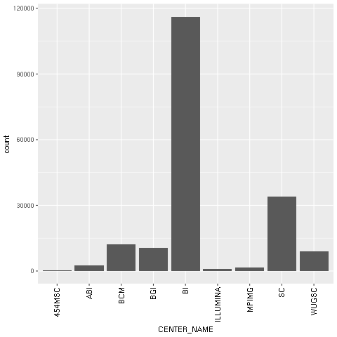
Figure 1: The ggplot2-generated histogram of center names, which is responsible for sequencing the lanes of the human genomic data from the 1,000 Genomes Project

robjects.r('yri_ceu <- seq.data[seq.data$POPULATION %in% c("YRI", "CEU") & seq.data$BASE_COUNT < 2E9 & seq.data$READ_COUNT < 3E7, ]')
yri_ceu=robjects.r('yri_ceu')

scatter = ggplot2.ggplot(yri_ceu) + ggplot2.aes_string(x='BASE_COUNT', y='READ_COUNT', shape='factor(POPULATION)', col='factor(ANALYSIS_GROUP)') + ggplot2.geom_point()
robjects.r.png('out.png')
scatter.plot()

Hopefully, this example (refer to the following screenshot) makes the power of the Grammar of Graphics approach clear. We will start by declaring the DataFrame and the type of chart in use (the scatter plot implemented by geom_point).

Note how easy it is to express that the shape of each point depends on the POPULATION variable and the color on the ANALYSIS_GROUP:

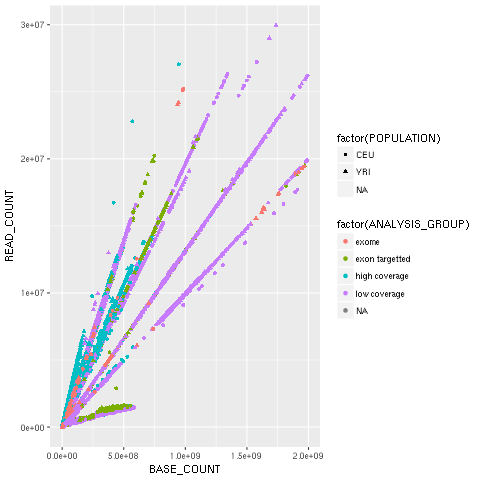
Figure 2: The ggplot2-generated scatter plot with base and read counts for all sequencing lanes read; the color and shape of each dot reflects categorical data (population and the type of data sequenced)

pd_yri_ceu = pandas2ri.ri2py(yri_ceu)
del pd_yri_ceu['PAIRED_FASTQ']
no_paired = pandas2ri.py2ri(pd_yri_ceu)
robjects.r.assign('no.paired', no_paired)
robjects.r("print(colnames(no.paired))")

We start by importing the necessary conversion module. We then convert the R DataFrame (note that we are converting yri_ceuin the R namespace, not the one on the Python namespace). We delete the column that indicates the name of the paired FASTQ file on the pandas DataFrame and copy it back to the R namespace. If you print the column names of the new R DataFrame, you will see thatPAIRED_FASTQis missing.

It's worth repeating that the advances in the Python software ecology are occurring at a breakneck pace. This means that if a certain functionality is not available today, it might be released sometime in the near future. So, if you are developing a new project, be sure to check for the very latest developments on the Python front before using functionality from an R package.

There are plenty of R packages for Bioinformatics in the Bioconductor project (http://www.bioconductor.org/). This should probably be your first port of call in the R world for bioinformatics functionalities. However, note that there are many R Bioinformatics packages that are not on Bioconductor, so be sure to search the wider R packages on Comprehensive R Archive Network (CRAN) (refer to CRAN at http://cran.rproject.org/).

There are plenty of plotting libraries for Python. Matplotlib is the most common library, but you also have a plethora of other choices. In the context of R, it's worth noting that there is a ggplot2-like implementation for Python based on the Grammar of Graphics description language for charts, and this is called—surprise, surprise—ggplot! (http://yhat.github.io/ggpy/).

You will need to follow the previous Getting ready steps of the Interfacing with R via rpy2 recipe. The Notebook is Chapter01/R_magic.ipynb. The Notebook is more complete than the recipe presented here, and includes more chart examples. For brevity here, we will only concentrate on the fundamental constructs to interact with R using magics.

This recipe is an aggressive simplification of the previous one because it illustrates the conciseness and elegance of R magics:

import rpy2.robjects as robjects
import rpy2.robjects.lib.ggplot2 as ggplot2%load_ext rpy2.ipython

Note that the % starts an IPython-specific directive. Just as a simple example, you can write %R print(c(1, 2)) on a Jupyter cell.

Check out how easy it is to execute the R code without using the robjects package. Actually, rpy2 is being used to look under the hood.

%%R
seq.data <- read.delim('sequence.index', header=TRUE, stringsAsFactors=FALSE)
seq.data$READ_COUNT <-as.integer(seq.data$READ_COUNT)
seq.data$BASE_COUNT <-as.integer(seq.data$BASE_COUNT)

You can then specify that the whole cell should be interpreted as an R code by using %%R (note the double %%).

seq_data = %R seq.data
print(type(seq_data))  # pandas dataframe!

The type of the DataFrame is not a standard Python object, but a pandas DataFrame. This is a departure from previous versions of the R magic interface.

my_col = list(seq_data.columns).index("CENTER_NAME")
seq_data['CENTER_NAME'] = seq_data['CENTER_NAME'].apply(lambda x: x.upper())

%R -i seq_data
%R print(colnames(seq_data))

The -i argument informs the magic system that the variable that follows on the Python space is to be copied in the R namespace. The second line just shows that the DataFrame is indeed available in R. The name that we are using is different from the original—it's seq_data instead of seq.data.

%%R
bar <- ggplot(seq_data) +  aes(factor(CENTER_NAME)) + geom_bar() + theme(axis.text.x = element_text(angle = 90, hjust = 1))
print(bar)

The R magic system also allows you to reduce code, as it changes the behavior of the interaction of R with IPython. For example, in the ggplot2 code of the previous recipe, you do not need to use the .png and dev.off R functions, as the magic system will take care of this for you. When you tell R to print a chart, it will magically appear in your Notebook or graphical console.

The R magics have seemed to have changed quite a lot over time in terms of interface. For example, I updated the R code for the first edition of this book a few times. The current version of DataFrame assignment returns pandas objects, which is a major change. Be careful with the version of Jupyter that you use as the %R code can be quite different. If this code does not work and you are using an older version, consult the Notebooks of the first edition of this book, as they might help.