Reader small image

You're reading from  The Applied Data Science Workshop - Second Edition

Product typeBook
Published inJul 2020
Reading LevelIntermediate
PublisherPackt
ISBN-139781800202504
Edition2nd Edition
Languages
Tools
Concepts
Right arrow
Author (1)
Alex Galea
Alex Galea
author image
Alex Galea

Alex Galea has been professionally practicing data analytics since graduating with a masters degree in physics from the University of Guelph, Canada. He developed a keen interest in Python while researching quantum gases as part of his graduate studies. Alex is currently doing web data analytics, where Python continues to play a key role in his work. He is a frequent blogger about data-centric projects that involve Python and Jupyter Notebooks.
Read more about Alex Galea

Right arrow

1. Introduction to Jupyter Notebooks

Overview

This chapter describes Jupyter Notebooks and their use in data analysis. It also explains the features of Jupyter Notebooks, which allow for additional functionality beyond running Python code. You will learn and implement the fundamental features of Jupyter Notebooks by completing several hands-on exercises. By the end of this chapter, you will be able to use some important features of Jupyter Notebooks and some key libraries available in Python.

Introduction

Our approach to learning in this book is highly applied since hands-on learning is the quickest way to understand abstract concepts. With this in mind, the focus of this chapter is to introduce Jupyter Notebooks—the data science tool that we will be using throughout this book.

Since Jupyter Notebooks have gained mainstream popularity, they have been one of the most important tools for data scientists who use Python. This is because they offer a great environment for a variety of tasks, such as performing quick and dirty analysis, researching model selection, and creating reproducible pipelines. They allow for data to be loaded, transformed, and modeled inside a single file, where it's quick and easy to test out code and explore ideas along the way. Furthermore, all of this can be documented inline using formatted text, which means you can make notes or even produce a structured report.

Other comparable platforms—for example, RStudio or Spyder—offer multiple panels to work between. Frequently, one of these panels will be a Read Eval Prompt Loop (REPL), where code is run on a Terminal session that has saved memory. Code written here may end up being copied and pasted into a different panel within the main codebase, and there may also be additional panels to see visualizations or other files. Such development environments are prone to efficiency issues and can promote bad practices for reproducibility if you're not careful.

Jupyter Notebooks work differently. Instead of having multiple panels for different components of your project, they offer the same functionality in a single component (that is, the Notebook), where the text is displayed along with code snippets, and code outputs are displayed inline. This lets you code efficiently and allows you to look back at previous work for reference, or even make alterations.

We'll start this chapter by explaining exactly what Jupyter Notebooks are and why they are so popular among data scientists. Then, we'll access a Notebook together and go through some exercises to learn how the platform is used.

Basic Functionality and Features of Jupyter Notebooks

In this section, we will briefly demonstrate the usefulness of Jupyter Notebooks with examples. Then, we'll walk through the basics of how they work and how to run them within the Jupyter platform. For those who have used Jupyter Notebooks before, this will be a good refresher, and you are likely to uncover new things as well.

What Is a Jupyter Notebook and Why Is It Useful?

Jupyter Notebooks are locally run on web applications that contain live code, equations, figures, interactive apps, and Markdown text in which the default programming language is Python. In other words, a Notebook will assume you are writing Python unless you tell it otherwise. We'll see examples of this when we work through our first workbook, later in this chapter.

Note

Jupyter Notebooks support many programming languages through the use of kernels, which act as bridges between the Notebook and the language. These include R, C++, and JavaScript, among many others. A list of available kernels can be found here: https://packt.live/2Y0jKJ0.

The following is an example of a Jupyter Notebook:

Figure 1.1: Jupyter Notebook sample workbook

Figure 1.1: Jupyter Notebook sample workbook

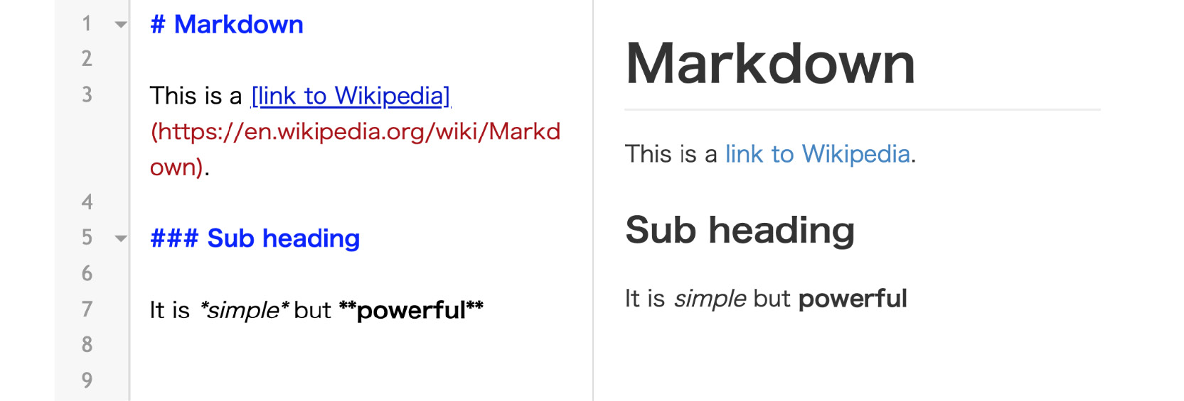
Besides executing Python code, you can write in Markdown to quickly render formatted text, such as titles, lists, or bold font. This can be done in combination with code using the concept of independent cells in the Notebook, as seen in Figure 1.2. Markdown is not specific to Jupyter; it is also a simple language used for styling text and creating basic documents. For example, most GitHub repositories have a README.md file that is written in Markdown format. It's comparable to HTML but offers much less customization in exchange for simplicity.

Commonly used symbols in markdown include hashes (#) to make text into a heading, square ([]) and round brackets (()) to insert hyperlinks, and asterisks (*) to create italicized or bold text:

Figure 1.2: Sample Markdown document

Figure 1.2: Sample Markdown document

In addition, Markdown can be used to render images and add hyperlinks in your document, both of which are supported in Jupyter Notebooks.

Jupyter Notebooks was not the first tool to use Markdown alongside code. This was the design of R Markdown, a hybrid language where R code can be written and executed inline with Markdown text. Jupyter Notebooks essentially offer the equivalent functionality for Python code. However, as we will see, they function quite differently from R Markdown documents. For example, R Markdown assumes you are writing Markdown unless otherwise specified, whereas Jupyter Notebooks assume you are inputting code. This and other features (as we will explore throughout) make it more appealing to use Jupyter Notebooks for rapid development in data science research.

While Jupyter Notebooks offer a blank canvas for a general range of applications, the types of Notebooks commonly seen in real-world data science can be categorized as either lab-style or deliverable.

Lab-style Notebooks serve as the programming analog of research journals. These should contain all the work you've done to load, process, analyze, and model the data. The idea here is to document everything you've done for future reference. For this reason, it's usually not advisable to delete or alter previous lab-style Notebooks. It's also a good idea to accumulate multiple date-stamped versions of the Notebook as you progress through the analysis, in case you want to look back at previous states.

Deliverable Notebooks are intended to be presentable and should contain only select parts of the lab-style Notebooks. For example, this could be an interesting discovery to share with your colleagues, an in-depth report of your analysis for a manager, or a summary of the key findings for stakeholders.

In either case, an important concept is reproducibility. As long as all the relevant software versions were documented at runtime, anybody receiving a Notebook can rerun it and compute the same results as before. The process of actually running code in a Notebook (as opposed to reading a pre-computed version) brings you much closer to the actual data. For example, you can add cells and ask your own questions regarding the datasets or tweak existing code. You can also experiment with Python to break down and learn about sections of code that you are struggling to understand.

Editing Notebooks with Jupyter Notebooks and JupyterLab

It's finally time for our first exercise. We'll start by exploring the interface of the Jupyter Notebook and the JupyterLab platforms. These are very similar applications for running Jupyter Notebook (.ipynb) files, and you can use whatever platform you prefer for the remainder of this book, or swap back and forth, once you've finished the following exercises.

Note

The .ipynb file extension is standard for Jupyter Notebooks, which was introduced back when they were called IPython Notebooks. These files are human-readable JSON documents that can be opened and modified with any text editor. However, there is usually no reason to open them with any software other than Juptyer Notebook or JupyterLab, as described in this section. Perhaps the one exception to this rule is when doing version control with Git, if you may want to see the changes in plain text.

At this stage, you'll need to make sure that you have the companion material downloaded. This can be downloaded from the open source repository on GitHub at https://packt.live/2zwhfom.

In order to run the code, you should download and install the Anaconda Python distribution for Python 3.7 (or a more recent version). If you already have Python installed and don't want to use Anaconda, you may choose to install the dependencies manually instead (see requirements.txt in the GitHub repository).

Note

Virtual environments are a great tool for managing multiple projects on the same machine. Each virtual environment may contain a different version of Python and external libraries. In addition to Python's built-in virtual environments, conda also offers virtual environments, which tend to integrate better with Jupyter Notebooks.

For the purposes of this book, you do not need to worry about virtual environments. This is because they add complexity that will likely lead to more issues than they aim to solve. Beginners are advised to run global system installs of Python libraries (that is, using the pip commands shown here). However, more experienced Python programmers might wish to create and activate a virtual environment for this project.

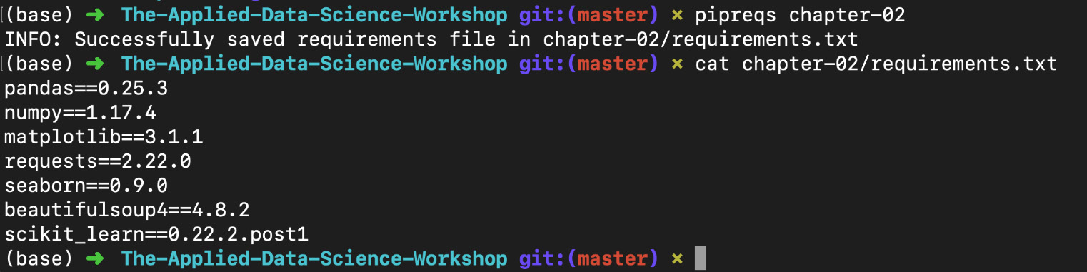
We will install additional Python libraries throughout this book, but it's recommended to install some of these (such as mlxtend, watermark, and graphviz) ahead of time if you have access to an internet connection now. This can be done by opening a new Terminal window and running the pip or conda commands, as follows:

  • mlxtend (https://packt.live/3ftcN98): This is a useful tool for particular data science tasks. We'll use it to visualize the decision boundaries of models in Chapter 5, Model Validation and Optimization, and Chapter 6, Web Scraping with Jupyter Notebooks:
    pip install mlxtend
  • watermark (https://packt.live/2N1qjok): This IPython magic extension is used for printing version information. We'll use it later in this chapter:
    pip install watermark
  • graphviz (https://packt.live/3hqqCHz): This is for rendering graph visualizations. We'll use this for visualizing decision trees in Chapter 5, Model Validation and Optimization:
    conda install -c anaconda graphviz python-graphviz

graphviz will only be used once, so don't worry too much if you have issues installing it. However, hopefully, you were able to get mlxtend installed since we'll need to rely on it in later chapters to compare models and visualize how they learn patterns in the data.

Exercise 1.01: Introducing Jupyter Notebooks

In this exercise, we'll launch the Jupyter Notebook platform from the Terminal and learn how the visual user interface works. Follow these steps to complete this exercise:

  1. Navigate to the companion material directory from the Terminal. If you don't have the code downloaded yet, you can clone it using the git command-line tool:
    git clone https://github.com/PacktWorkshops/The-Applied-Data-Science-Workshop.git
    cd The-Applied-Data-Science-Workshop

    Note

    With Unix machines such as Mac or Linux, command-line navigation can be done using ls to display directory contents and cd to change directories. On Windows machines, use dir to display directory contents and use cd to change directories. If, for example, you want to change the drive from C: to D:, you should execute D: to change drives. This is an important step if you wish to enable all commands based on folder structure and ensure they run smoothly.

  2. Run the Jupyter Notebook platform by asking for its version:

    Note

    The # symbol in the code snippet below denotes a code comment. Comments are added into code to help explain specific bits of logic.

    jupyter notebook –-version
    # should return 6.0.2 or a similar / more recent version
  3. Start a new local Notebook server here by typing the following into the Terminal:
    jupyter notebook

    A new window or tab of your default browser will open the Notebook Dashboard to the working directory. Here, you will see a list of folders and files contained therein.

  4. Reopen the Terminal window that you used to launch the app. We will see the NotebookApp being run on a local server. In particular, you should see a line like this in the Terminal:
    [I 20:03:01.045 NotebookApp] The Jupyter Notebook is running at: http:// localhost:8888/?token=e915bb06866f19ce462d959a9193a94c7 c088e81765f9d8a

    Going to the highlighted HTTP address will load the app in your browser window, as was done automatically when starting the app.

  5. Reopen the web browser and play around with the Jupyter Dashboard platform by clicking on a folder (such as chapter-06), and then clicking on an .ipynb file (such as chapter_6_workbook.ipynb) to open it. This will cause the Notebook to open in a new tab on your browser.
  6. Go back to the tab on your browser that contains the Jupyter Dashboard. Then, go back to the root directory by clicking the button (above the folder content listing) or the folder icon above that (in the current directory breadcrumb).
  7. Although its main use is for editing Notebook files, Jupyter is a basic text editor as well. To see this, click on the requirements.txt text file. Similar to the Notebook file, it will open in a new tab of your browser.
  8. Now, you need to close the platform. Reopen the Terminal window you used to launch the app and stop the process by typing Ctrl + C in the Terminal. You may also have to confirm this by entering y and pressing Enter. After doing this, close the web browser window as well.
  9. Now, you are going to explore the Jupyter Notebook command-line interface (CLI) a bit. Load the list of available options by running the following command:
    jupyter notebook --help
  10. One option is to specify the port for the application to run on. Open the NotebookApp at local port 9000 by running the following command:
    jupyter notebook --port 9000
  11. Click New in the upper right-hand corner of the Jupyter Dashboard and select a kernel from the drop-down menu (that is, select something in the Notebooks section):
    Figure 1.3: Selecting a kernel from the drop-down menu

    Figure 1.3: Selecting a kernel from the drop-down menu

    This is the primary method of creating a new Jupyter Notebook.

    Kernels provide programming language support for the Notebook. If you have installed Python with Anaconda, that version should be the default kernel. Virtual environments that have been properly configured will also be available here.

  12. With the newly created blank Notebook, click the top cell and type print('hello world'), or any other code snippet that writes to the screen.
  13. Click the cell and press Shift + Enter or select Run Cell from the Cell menu.

    Any stdout or stderr output from the code will be displayed beneath as the cell runs. Furthermore, the string representation of the object written in the final line will be displayed as well. This is very handy, especially for displaying tables, but sometimes, we don't want the final object to be displayed. In such cases, a semicolon (;) can be added to the end of the line to suppress the display. New cells expect and run code input by default; however, they can be changed to render markdown instead.

  14. Click an empty cell and change it to accept the Markdown-formatted text. This can be done from the drop-down menu icon in the toolbar or by selecting Markdown from the Cell menu. Write some text in here (any text will do), making sure to utilize Markdown formatting symbols such as #, and then run the cell using Shift + Enter:
    Figure 1.4: Menu options for converting cells into code/Markdown

    Figure 1.4: Menu options for converting cells into code/Markdown

  15. Scroll to the Run button in the toolbar:
    Figure 1.5: Toolbar icon to start cell execution

    Figure 1.5: Toolbar icon to start cell execution

  16. This can be used to run cells. As you will see later, however, it's handier to Shift + Enter to run cells.
  17. Right next to the Run button is a Stop icon, which can be used to stop cells from running. This is useful, for example, if a cell is taking too long to run:
    Figure 1.6: Toolbar icon to stop cell execution

    Figure 1.6: Toolbar icon to stop cell execution

  18. New cells can be manually added from the Insert menu:
    Figure 1.7: Menu options for adding new cells

    Figure 1.7: Menu options for adding new cells

  19. Cells can be copied, pasted, and deleted using icons or by selecting options from the Edit menu:
    Figure 1.8: Toolbar icons to cut, copy, and paste cells

    Figure 1.8: Toolbar icons to cut, copy, and paste cells

    The drop-down list from the Edit menu is as follows:

    Figure 1.9: Menu options to cut, copy, and paste cells

    Figure 1.9: Menu options to cut, copy, and paste cells

  20. Cells can also be moved up and down this way:
    Figure 1.10: Toolbar icons for moving cells up or down

    Figure 1.10: Toolbar icons for moving cells up or down

    There are useful options in the Cell menu that you can use to run a group of cells or the entire Notebook:

    Figure 1.11: Menu options for running cells in bulk

    Figure 1.11: Menu options for running cells in bulk

    Experiment with the toolbar options to move cells up and down, insert new cells, and delete cells. An important thing to understand about these Notebooks is the shared memory between cells. It's quite simple; every cell that exists on the sheet has access to the global set of variables. So, for example, a function defined in one cell could be called from any other, and the same applies to variables. As you would expect, anything within the scope of a function will not be a global variable and can only be accessed from within that specific function.

  21. Open the Kernel menu to see the selections. The Kernel menu is useful for stopping the execution of the script and restarting the Notebook if the kernel dies:
    Figure 1.12: Menu options for selecting a Notebook kernel

    Figure 1.12: Menu options for selecting a Notebook kernel

    Kernels can also be swapped here at any time, but it is inadvisable to use multiple kernels for a single Notebook due to reproducibility concerns.

  22. Open the File menu to see the selections. The File menu contains options for downloading the Notebook in various formats. It's recommended to save an HTML version of your Notebook, where the content is rendered statically and can be opened and viewed as you would expect in web browsers.
  23. The Notebook name will be displayed in the upper left-hand corner. New Notebooks will automatically be named Untitled. You can change the name of your .ipynb Notebook file by clicking on the current name in the upper left corner and typing in the new name. Then, save the file.
  24. Close the current tab in your web browser (exiting the Notebook) and go to the Jupyter Dashboard tab, which should still be open. If it's not open, then reload it by copying and pasting the HTTP link from the Terminal.
  25. Since you didn't shut down the Notebook (you just saved and exited it), it will have a green book symbol next to its name in the Files section of the Jupyter Dashboard, and it will be listed as Running on the right-hand side next to the last modified date. Notebooks can be shut down from here.
  26. Quit the Notebook you have been working on by selecting it (checkbox to the left of the name) and clicking the orange Shutdown button.

    Note

    If you plan to spend a lot of time working with Jupyter Notebooks, it's worthwhile learning the keyboard shortcuts. This will speed up your workflow considerably. Particularly useful commands to learn are the shortcuts for manually adding new cells and converting cells from code into Markdown formatting. Click on Keyboard Shortcuts from the Help menu to see how.

  27. Go back to the Terminal window that's running the Jupyter Notebook server and shut it down by typing Ctrl + C. Confirm this operation by typing y and pressing Enter. This will automatically exit any kernel that is running. Do this now and close the browser window as well.

Now that we have learned the basics of Jupyter Notebooks, we will launch and explore the JupyterLab platform.

While the Jupyter Notebook platform is lightweight and simple by design, JupyterLab is closer to R Studio in design. In JupyterLab, you can stack notebooks side by side, along with console environments (REPLs) and data tables, among other things you may want to look at.

Although the new features it provides are nice, the simplicity of the Jupyter Notebook interface means that it's still an appealing choice. Aside from its simplicity, you may find the Jupyter Notebook platform preferable for the following reasons:

  • You may notice minor latency issues in JupyterLab that are not present in the Jupyter Notebook platform.
  • JupyterLab can be extremely slow to load large .ipynb files (this is an open issue on GitHub, as of early 2020).

Please don't let these small issues hold you back from trying out JupyterLab. In fact, it would not be surprising if you decide to use it for running the remainder of the exercises and activities in this book.

The future of open source tooling around Python and data science is going to be very exciting, and there are sure to be plenty of developments regarding Jupyter tools in the years to come. This is all thanks to the open source programmers who build and maintain these projects and the companies that contribute to the community.

Exercise 1.02: Introducing the JupyterLab Platform

In this exercise, we'll launch the JupyterLab platform and see how it compares with the Jupyter Notebook platform.

Follow these steps to complete this exercise:

  1. Run JupyterLab by asking for its version:
    jupyter lab --version
    # should return 1.2.3 or a similar / more recent version
  2. Navigate to the root directory, and then, launch JupyterLab by typing the following into the Terminal:
    jupyter lab

    Similar to when we ran the Jupyter Notebook server, a new window or tab on your default browser should open the JupyterLab Dashboard. Here, you will see a list of folders and files in the working directory in a navigation bar to the left:

    Figure 1.13: JupyterLab dashboard

    Figure 1.13: JupyterLab dashboard

  3. Looking back at the Terminal, you can see a very similar output to what our NotebookApp showed us before, except now for the LabApp. If nothing else is running there, it should launch on port 8888 by default:
    [I 18:37:29.369 LabApp] The Jupyter Notebook is running at:
    [I 18:37:29.369 LabApp] http://localhost:8888/?token=cb55c8f3c03f0d6843ae59e70bedbf3b6ec 4a92288e65fa3
  4. Looking back at the browser window, you can see that the JupyterLab Dashboard has many of the same menus as the Jupyter Notebook platform. Open a new Notebook by clicking File | New | Notebook:
    Figure 1.14: Opening a new notebook

    Figure 1.14: Opening a new notebook

  5. When prompted to select a kernel, choose Python 3:
    Figure 1.15: Selecting a kernel for our notebook

    Figure 1.15: Selecting a kernel for our notebook

    The Notebook will then load into a new tab inside JupyterLab. Notice how this is different from the Jupyter Notebook platform, where each file is opened in its own browser tab.

  6. You will see that a toolbar has appeared at the top of the tab, with the buttons we previously explored, such as those to save, run, and stop code:
    Figure 1.16: JupyterLab toolbar and Notebook tab

    Figure 1.16: JupyterLab toolbar and Notebook tab

  7. Run the following code in the first cell of the Notebook to produce some output in the space below by Shift + Enter:
    for i in range(10):
        print(i, i % 3)

    This will look as follows in Jupyter Notebook:

    Figure 1.17: Output of the for loop

    Figure 1.17: Output of the for loop

  8. When you place your mouse pointer in the white space present to the left of the cell, you will see two blue bars appear to the left of the cell. This is one of JupyterLab's new features. Click on them to hide the code cell or its output:
    Figure 1.18: Bars that hide/show cells and output in JupyterLab

    Figure 1.18: Bars that hide/show cells and output in JupyterLab

  9. Explore window stacking in JupyterLab. First, save your new Notebook file by clicking File | Save Notebook As and giving it the name test.ipynb:
    Figure 1.19: Prompt for saving the name of the file

    Figure 1.19: Prompt for saving the name of the file

  10. Click File | New | Console in order to load up a Python interpreter session:
    Figure 1.20: Opening a new console session

    Figure 1.20: Opening a new console session

  11. This time, when you see the kernel prompt, select test.ipynb under Use Kernel from Other Session. This feature of JupyterLab allows each process to have shared access to variables in memory:
    Figure 1.21: Electing the console kernel

    Figure 1.21: Electing the console kernel

  12. Click on the new Console window tab and drag it down to the bottom half of the screen in order to stack it underneath the Notebook. Now, define something in the console session, such as the following:
    a = 'apple'

    It will look as follows:

    Figure 1.22: Split view of the Notebook and console in JupyterLab

    Figure 1.22: Split view of the Notebook and console in JupyterLab

  13. Run this cell with Shift + Enter (or using the Run menu), and then run another cell below to test that your variable returns the value as expected; for example, print(a).
  14. Since you are using a shared kernel between this console and the Notebook, click into a new cell in the test.ipynb Notebook and print the variable there. Test that this works as expected; for example, print(a):
    Figure 1.23: Sharing a kernel between processes in JupyterLab

    Figure 1.23: Sharing a kernel between processes in JupyterLab

    A great feature of JupyterLab is that you can open up and work on multiple views of the same Notebook concurrently—something that cannot be done with the Jupyter Notebook platform. This can be very useful when working in large Notebooks where you want to frequently look at different sections.

  15. You can work on multiple views of test.ipynb by right-clicking on its tab and selecting New View for Notebook:
    Figure 1.24: Opening a new view for an open Notebook

    Figure 1.24: Opening a new view for an open Notebook

    You should see a copy of the Notebook open to the right. Now, start typing something into one of the cells and watch the other view update as well:

    Figure 1.25: Two live views of the same Notebook in JupyterLab

    Figure 1.25: Two live views of the same Notebook in JupyterLab

    There are plenty of other neat features in JupyterLab that you can discover and play with. For now, though, we are going to close down the platform.

  16. Click the circular button with a box in the middle on the far left-hand side of the Dashboard. This will pull up a panel showing the kernel sessions open right now. You can click SHUT DOWN to close anything that is open:
    Figure 1.26: Shutting down Notebook sessions in JupyterLab

    Figure 1.26: Shutting down Notebook sessions in JupyterLab

  17. Go back to the Terminal window that's running the JupyterLab server and shut it down by pressing Ctrl + C, then confirm the operation by pressing Y and pressing Enter. This will automatically exit any kernel that is running. Do this now and close the browser window as well:
    Figure 1.27: Shutting down the LabApp

Figure 1.27: Shutting down the LabApp

In this exercise, we learned about the JupyterLab platform and how it compares to the older Jupyter Notebook platform for running Notebooks. In addition to learning about the basics of using the app, we explored some of its awesome features, all of which can help your data science workflow.

In the next section, we'll learn about some of the more general features of Jupyter that apply to both platforms.

Jupyter Features

Having familiarized ourselves with the interface of two platforms for running Notebooks (Jupyter Notebook and JupyterLab), we are ready to start writing and running some more interesting examples.

Note

For the remainder of this book, you are welcome to use either the Jupyter Notebook platform or JupyterLab to follow along with the exercises and activities. The experience is similar, and you will be able to follow along seamlessly either way. Most of the screenshots for the remainder of this book have been taken from JupyterLab.

Jupyter has many appealing core features that make for efficient Python programming. These include an assortment of things, such as tab completion and viewing docstrings—both of which are very handy when writing code in Jupyter. We will explore these and more in the following exercise.

Note

The official IPython documentation can be found here: https://ipython.readthedocs.io/en/stable/. It provides details of the features we will discuss here, as well as others.

Exercise 1.03: Demonstrating the Core Jupyter Features

In this exercise, we'll relaunch the Jupyter platform and walk through a Notebook to learn about some core features, such as navigating workbooks with keyboard shortcuts and using magic functions. Follow these steps to complete this exercise:

  1. Start up one of the following platforms for running Jupyter Notebooks:

    JupyterLab (run jupyter lab)

    Jupyter Notebook (run jupyter notebook)

    Then, open the platform in your web browser by copying and pasting the URL, as prompted in the Terminal.

    Note

    Here's the list of basic keyboard shortcuts; these are especially helpful if you wish to avoid having to use the mouse so often, which will greatly speed up your workflow.

    Shift + Enter to run a cell

    Esc to leave a cell

    a to add a cell above

    b to add a cell below

    dd to delete a cell

    m to change a cell to Markdown (after pressing Esc)

    y to change a cell to code (after pressing Esc)

    Arrow keys to move cells (after pressing Esc)

    Enter to enter a cell

    You can get help by adding a question mark to the end of any object and running the cell. Jupyter finds the docstring for that object and returns it in a pop-up window at the bottom of the app.

  2. Import numpy and get the arrange docstring, as follows:
    import numpy as np
    np.arange?

    The output will be similar to the following:

    Figure 1.28: The docstring for np.arange

    Figure 1.28: The docstring for np.arange

  3. Get the Python sorted function docstring as follows:
    sorted?

    The output is as follows:

    Figure 1.29: The docstring for sort

    Figure 1.29: The docstring for sort

  4. You can pull up a list of the available functions on an object. You can do this for a NumPy array by running the following command:
    a = np.array([1, 2, 3])
    a.*?

    Here's the output showing the list:

    Figure 1.30: The output after running a.*?

    Figure 1.30: The output after running a.*?

  5. Click an empty code cell in the Tab Completion section. Type import (including the space after) and then press the Tab key:
    import <tab>

    Tab completion can be used to do the following:

  6. List the available modules when importing external libraries:
    from numpy import <tab>
  7. List the available modules of imported external libraries:
    np.<tab>
  8. Perform function and variable completion:
    np.ar<tab>
    sor<tab>([2, 3, 1])
    myvar_1 = 5
    myvar_2 = 6
    my<tab>

    Test each of these examples for yourself in the following cells:

    Figure 1.31: An example of tab completion for variable names

    Figure 1.31: An example of tab completion for variable names

    Note

    Tab completion is different in the JupyterLab and Jupyter Notebook platforms. The same commands may not work on both.

    Tab completion can be especially useful when you need to know the available input arguments for a module, explore a new library, discover new modules, or simply speed up the workflow. They will save time writing out variable names or functions and reduce bugs from typos. Tab completion works so well that you may have difficulty coding Python in other editors after today.

  9. List the available magic commands, as follows:
    %lsmagic

    The output is as follows:

    Figure 1.32: Jupyter magic functions

    Figure 1.32: Jupyter magic functions

    Note

    If you're running JupyterLab, you will not see the preceding output. A list of magic functions, along with information about each, can be found here: https://ipython.readthedocs.io/en/stable/interactive/magics.html.

    The percent signs, % and %%, are one of the basic features of Jupyter Notebook and are called magic commands. Magic commands starting with %% will apply to the entire cell, while magic commands starting with % will only apply to that line.

  10. One example of a magic command that you will see regularly is as follows. This is used to display plots inline, which avoids you having to type plt.show() each time you plot something. You only need to execute it once at the beginning of the session:
    %matplotlib inline

    The timing functions are also very handy magic functions and come in two varieties: a standard timer (%time or %%time) and a timer that measures the average runtime of many iterations (%timeit and %%timeit). We'll see them being used here.

  11. Declare the a variable, as follows:
    a = [1, 2, 3, 4, 5] * int(1e5)
  12. Get the runtime for the entire cell, as follows:
    %%time
    for i in range(len(a)):
        a[i] += 5

    The output is as follows:

    CPU times: user 68.8 ms, sys: 2.04 ms, total: 70.8 ms
    Wall time: 69.6 ms
  13. Get the runtime for one line:
    %time a = [_a + 5 for _a in a]

    The output is as follows:

    CPU times: user 21.1 ms, sys: 2.6 ms, total: 23.7 ms
    Wall time: 23.1 ms
  14. Check the average results of multiple runs, as follows:
    %timeit set(a)

    The output is as follows:

    4.72 ms ± 55.5 µs per loop (mean ± std. dev. of 7 runs, 100 loops each)

    Note the difference in use between one and two percent signs. Even when using a Python kernel (as you are currently doing), other languages can be invoked using magic commands. The built-in options include JavaScript, R, Perl, Ruby, and Bash. Bash is particularly useful as you can use Unix commands to find out where you are currently (pwd), see what's in the directory (ls), make new folders (mkdir), and write file contents (cat/head/tail).

    Note

    Notice how list comprehensions are quicker than loops in Python. This can be seen by comparing the wall time for the first and second cell, where the same calculation is done significantly faster with list comprehension. Please note that the step 15-18 are Linux-based commands. If you are working on other operating systems like Windows and MacOS, these steps might not work.

  15. Write some text into a file in the working directory, print the directory's contents, print an empty line, and then write back the contents of the newly created file before removing it, as follows:
    %%bash
    echo "using bash from inside Jupyter!" > test-file.txt
    ls
    echo ""
    cat test-file.txt
    rm test-file.txt

    The output is as follows:

    Figure 1.33: Running a bash command in Jupyter

    Figure 1.33: Running a bash command in Jupyter

  16. List the contents of the working directory with ls, as follows:
    %ls

    The output is as follows:

    chapter_1_workbook.ipynb
  17. List the path of the current working directory with pwd. Notice how we needed to use the %%bash magic function for pwd, but not for ls:
    %%bash
    pwd

    The output is as follows:

    /Users/alex/Documents/The-Applied-Data-Science-Workshop/chapter-01
  18. There are plenty of external magic commands that can be installed. A popular one is ipython-sql, which allows for SQL code to be executed in cells.

    Jupyter magic functions can be installed the same way as PyPI Python libraries, using pip or conda. Open a new Terminal window and execute the following code to install ipython-sql:

    pip install ipython-sql
  19. Run the %load_ext sql cell to load the external command into the Notebook.

    This allows connections to be made to remote databases so that queries can be executed (and thereby documented) right inside the Notebook.

  20. Now, run the sample SQL query, as follows:
    %%sql sqlite://
    SELECT *
    FROM (
        SELECT 'Hello' as msg1, 'World!' as msg2
    );

    The output is as follows:

    Figure 1.34: Running a SQL query in Jupyter

    Figure 1.34: Running a SQL query in Jupyter

    Here, we connected to the local sqlite source with sqlite://; however, this line could instead point to a specific database on a local or remote server. For example, a .sqlite database file on your desktop could be connected to with the line %sql sqlite:////Users/alex/Desktop/db.sqlite, where the username in this case is alex and the file is db.sqlite.

    After connecting, we execute a simple SELECT command to show how the cell has been converted to run SQL code instead of Python.

  21. Earlier in this chapter, we went over the instructions for installing the watermark external library, which helps to document versioning in the Notebook. If you haven't installed it yet, then open a new window and run the following code:
    pip install watermark

    Once installed, it can be imported into any Notebook using %load_ext watermark. Then, it can be used to document library versions and system hardware.

  22. Load and call the watermark magic function and call its docstring with the following command:
    %load_ext watermark
    %watermark?

    The output is as follows:

    Figure 1.35: The docstring for watermark

    Figure 1.35: The docstring for watermark

    Notice the various arguments that can be passed in when calling it, such as -a for author, -v for the Python version, -m for machine information, and -d for date.

  23. Use the watermark library to add version information to the notebook, as follows:

    Note

    The code snippet shown here uses a backslash ( \ ) to split the logic across multiple lines. When the code is executed, Python will ignore the backslash, and treat the code on the next line as a direct continuation of the current line.

    %watermark -d -v -m -p \
    requests,numpy,pandas,matplotlib,seaborn,sklearn

    The output is as follows:

    Figure 1.36: watermark output in the Notebook

Figure 1.36: watermark output in the Notebook

Note

To access the source code for this specific section, please refer to https://packt.live/30KoAfu.

You can also run this example online at https://packt.live/2Y49zTQ.

In this exercise, we looked at the core features of Jupyter, including tab completion and magic functions. You'll review these features and have a chance to test them out yourself in the activity at the end of this chapter.

Converting a Jupyter Notebook into a Python Script

In this section, we'll learn how to convert a Jupyter Notebook into a Python script. This is equivalent to copying and pasting the contents of each code cell into a single .py file. The Markdown sections are also included as comments.

It can be beneficial to convert a Notebook into a .py file because the code is then available in plain text format. This can be helpful for version control— to see the difference in code between two versions of a Notebook, for example. It can also be a helpful trick for extracting chunks of code.

This conversion can be done from the Jupyter Dashboard (File -> Download as) or by opening a new Terminal window, navigating to the chapter-02 folder, and executing the following:

jupyter nbconvert --to=python chapter_2_workbook.ipynb

The output is as follows:

Figure 1.37: Converting a Notebook into a script (.py) file

Figure 1.37: Converting a Notebook into a script (.py) file

Note that we are using the next chapter's Notebook for this example.

Another benefit of converting Notebooks into .py files is that, when you want to determine the Python library requirements for a Notebook, the pipreqs tool will do this for us, and export them into a requirements.txt file. This tool can be installed by running the following command:

pip install pipreqs

You might require root privileges for this.

This command is called from outside the folder containing your .py files. For example, if the .py files are inside a folder called chapter-02, you could do the following:

pipreqs chapter-02/

The output is as follows:

Figure 1.38: Using pipreqs to generate a requirements.txt file

Figure 1.38: Using pipreqs to generate a requirements.txt file

The resulting requirements.txt file for chapter_2_workbook.ipynb will look similar to the following:

cat chapter-02/requirements.txt
matplotlib==3.1.1
seaborn==0.9.0
numpy==1.17.4
pandas==0.25.3
requests==2.22.0
beautifulsoup4==4.8.1
scikit_learn==0.22

Python Libraries

Having now seen all the basics of Jupyter Notebooks, and even some more advanced features, we'll shift our attention to the Python libraries we'll be using in this book.

Libraries, in general, extend the default set of Python functions. Some examples of commonly used standard libraries are datetime, time, os, and sys. These are called standard libraries because they are included with every installation of Python.

For data science with Python, the most heavily relied upon libraries are external, which means they do not come as standard with Python.

The external data science libraries we'll be using in this book are numpy, pandas, seaborn, matplotlib, scikit-learn, requests, and bokeh.

Note

It's a good idea to import libraries using industry standards—for example, import numpy as np. This way, your code is more readable. Try to avoid doing things such as from numpy import *, as you may unwittingly overwrite functions. Furthermore, it's often nice to have modules linked to the library via a dot (.) for code readability.

Let's briefly introduce each:

  • numpy offers multi-dimensional data structures (arrays) that operations can be performed on. This is far quicker than standard Python data structures (such as lists). This is done in part by performing operations in the background using C. NumPy also offers various mathematical and data manipulation functions.
  • pandas is Python's answer to the R DataFrame. It stores data in 2D tabular structures where columns represent different variables and rows correspond to samples. pandas provides many handy tools for data wrangling, such as filling in NaN entries and computing statistical descriptions of the data. Working with pandas DataFrames will be a big focus of this book.
  • matplotlib is a plotting tool inspired by the MATLAB platform. Those familiar with R can think of it as Python's version of ggplot. It's the most popular Python library for plotting figures and allows for a high level of customization.
  • seaborn works as an extension of matplotlib, where various plotting tools that are useful for data science are included. Generally speaking, this allows for analysis to be done much faster than if you were to create the same things manually with libraries such as matplotlib and scikit-learn.
  • scikit-learn is the most commonly used machine learning library. It offers top-of-the-line algorithms and a very elegant API where models are instantiated and then fit with data. It also provides data processing modules and other tools that are useful for predictive analytics.
  • requests is the go-to library for making HTTP requests. It makes it straightforward to get HTML from web pages and interface with APIs. For parsing HTML, many choose BeautifulSoup4, which we'll cover in Chapter 6, Web Scraping with Jupyter Notebooks.

We'll start using these libraries in the next chapter.

Activity 1.01: Using Jupyter to Learn about pandas DataFrames

We are going to be using pandas heavily in this book. In particular, any data that's loaded into our Notebooks will be done using pandas. The data will be contained in a DataFrame object, which can then be transformed and saved back to disk afterward. These DataFrames offer convenient methods for running calculations over the data for exploration, visualization, and modeling.

In this activity, you'll have the opportunity to use pandas DataFrames, along with the Jupyter features that have been discussed in this section. Follow these steps to complete this activity:

  1. Start up one of the platforms for running Jupyter Notebooks and open it in your web browser by copying and pasting the URL, as prompted in the Terminal.

    Note

    While completing this activity, you will need to use many cells in the Notebook. Please insert new cells as required.

  2. Import the pandas and NumPy libraries and assign them to the pd and np variables, respectively.
  3. Pull up the docstring for pd.DataFrame. Scan through the Parameters section and read the Examples section.
  4. Create a dictionary with fruit and score keys, which correspond to list values with at least three items in each. Ensure that you give your dictionary a suitable name (note that in Python, a dictionary is a collection of values); for example, {"fruit": ["apple", ...], "score": [8, ...]}.
  5. Use this dictionary to create a DataFrame. You can do this using pd.DataFrame(data=name of dictionary). Assign it to the df variable.
  6. Display this DataFrame in the Notebook.
  7. Use tab completion to pull up a list of functions available for df.
  8. Pull up the docstring for the sort_values DataFrame function and read through the Examples section.
  9. Sort the DataFrame by score in descending order. Try to see how many times you can use tab completion as you write the code.
  10. Use the timeit magic function to test how long this sorting operation takes.

    Note

    The detailed steps for this activity, along with the solutions, can be found via this link

Summary

In this chapter, we've gone over the basics of using Jupyter Notebooks for data science. We started by exploring the platform and finding our way around the interface. Then, we discussed the most useful features, which include tab completion and magic functions. Finally, we introduced the Python libraries we'll be using in this book.

As we'll see in the coming chapters, these libraries offer high-level abstractions that allow data science to be highly accessible with Python. This includes methods for creating statistical visualizations, building data cleaning pipelines, and training models on millions of data points and beyond.

While this chapter focused on the basics of Jupyter platforms, the next chapter is where the real data science begins. The remainder of this book is very interactive, and in Chapter 3, Preparing Data for Predictive Modeling, we'll perform an analysis of housing data using Jupyter Notebook and the Seaborn plotting library.

lock icon
The rest of the chapter is locked
You have been reading a chapter from
The Applied Data Science Workshop - Second Edition
Published in: Jul 2020Publisher: PacktISBN-13: 9781800202504
Register for a free Packt account to unlock a world of extra content!
A free Packt account unlocks extra newsletters, articles, discounted offers, and much more. Start advancing your knowledge today.
undefined
Unlock this book and the full library FREE for 7 days
Get unlimited access to 7000+ expert-authored eBooks and videos courses covering every tech area you can think of
Renews at $15.99/month. Cancel anytime

Author (1)

author image
Alex Galea

Alex Galea has been professionally practicing data analytics since graduating with a masters degree in physics from the University of Guelph, Canada. He developed a keen interest in Python while researching quantum gases as part of his graduate studies. Alex is currently doing web data analytics, where Python continues to play a key role in his work. He is a frequent blogger about data-centric projects that involve Python and Jupyter Notebooks.
Read more about Alex Galea