


Introducing the A* Algorithm
A* is a complete and optimal heuristic search algorithm that finds the shortest possible path between the current game state and the winning state. The definition of complete and optimal in this state are as follows:
- Complete means that A* always finds a solution.
- Optimal means that A* will find the best solution.
To set up the A* algorithm, we need the following:
- An initial state
- A description of the goal states
- Admissible heuristics to measure progress toward the goal state
- A way to generate the next steps toward the goal
Once the setup is complete, we execute the A* algorithm using the following steps on the initial state:
- We generate all possible next steps.
- We store these children in the order of their distance from the goal.
- We select the child with the best score first and repeat these three steps on the child with the best score as the initial state. This is the shortest path to get to a node from the starting node.
Let's take, for example, the following figure:
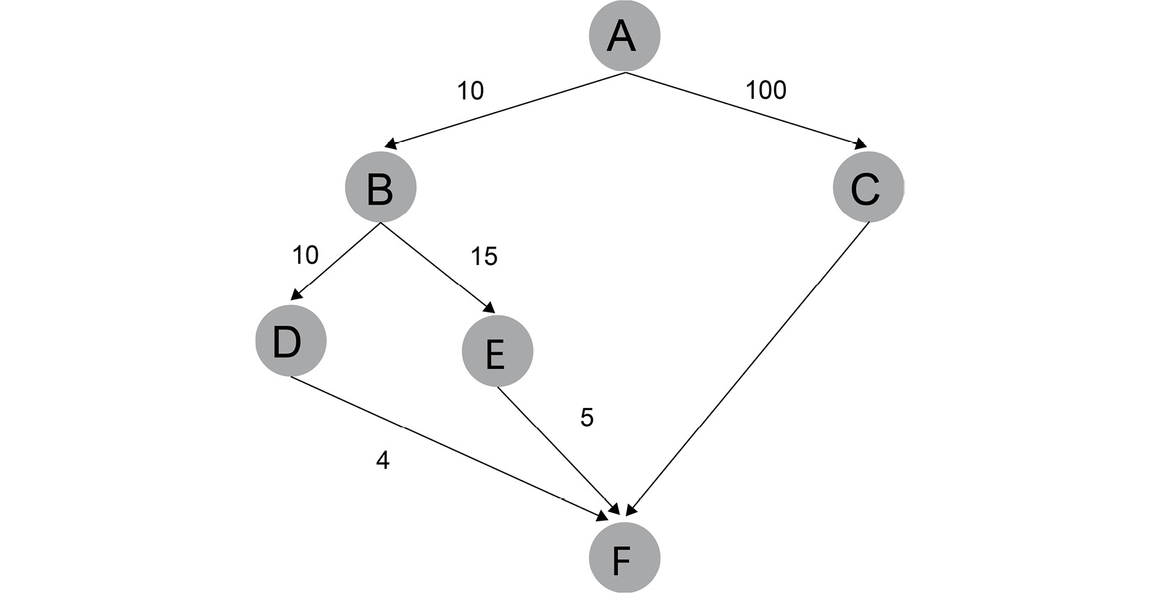
Figure 1.15: Tree with heuristic distance
The first step will be to generate all the possible moves from the origin, A, which is moving from A to B (A,B) or to C (A,C).
The second step is to use the heuristic (the distance) to order the two possible moves, (A,B), with 10, which is shorter compared to (A,C) with 100.
The third step is to choose the shortest heuristic, which is (A,B), and move to B.
Now, we will repeat the same steps with B as the origin.
At the end, we will reach the goal F with the path (A,B,D,F) with a cumulative heuristic of 24. If we were following another path, such as (A,B,E,F), the cumulative heuristic will be 30, which is higher than the shortest path.
We did not even look at (A,C,F) as it was already way over the shortest path.
In pathfinding, a good heuristic is the Euclidean distance. If the current node is (x, y) and the goal node is (u, v), then we have the following:
distance_from_end( node ) = sqrt( abs( x – u ) ** 2 + abs( y – v ) ** 2 )
Here, distance_from_end(node) is an admissible heuristic estimation showing how far we are from the goal node.
We also have the following:
sqrtis the square root function. Do not forget to import it from themathlibrary.absis the absolute value function, that is,abs( -2 ) = abs( 2 ) = 2.x ** 2isxraised to the second power.
We will use the distance_from_start matrix to store the distances from the start node. In the algorithm, we will refer to this cost matrix as distance_from_start(n1). For any node, n1, that has coordinates (x1, y1), this distance is equivalent to distance_from_start[x1][y1].
We will use the succ(n) notation to generate a list of successor nodes from n.
Note
The # symbol in the code snippet below denotes a code comment. Comments are added into code to help explain specific bits of logic. The triple-quotes ( """ ) shown in the code snippet below are used to denote the start and end points of a multi-line code comment. Comments are added into code to help explain specific bits of logic.
Have a look at the pseudocode of the algorithm:
frontier = [start], internal = {}
# Initialize the costs matrix with each cell set to infinity.
# Set the value of distance_from_start(start) to 0.
while frontier is not empty:
    """
    notice n has the lowest estimated total
    distance between start and end.
    """
    n = frontier.pop()
    # We'll learn later how to reconstruct the shortest path
    if n == end:
        return the shortest path.
    internal.add(n)
    for successor s in succ(n):
        if s in internal:
            continue # The node was already examined
        new_distance = distance_from_start(n) + distance(n, s)
        if new_distance >= distance_from_start(s):
            """
            This path is not better than the path we have
            already examined.
            """
            continue
        if s is a member of frontier:
            update the priority of s
        else:
            Add s to frontier.
Regarding the retrieval of the shortest path, we can use the costs matrix. This matrix contains the distance of each node on the path from the start node. As cost always decreases when walking backward, all we need to do is start with the end node and walk backward greedily toward decreasing costs:
path = [end_node], distance = get_distance_from_start( end_node )
while the distance of the last element in the path is not 0:
    for each neighbor of the last node in path:
        new_distance = get_distance_from_start( neighbor )
        if new_distance < distance:
            add neighbor to path, and break out from the for loop
return path
A* shines when we have one start state and one goal state. The complexity of the A* algorithm is O( E ), where E stands for all possible edges in the field. In our example, we have up to four edges leaving any node: up, down, left, and right.
Note
To sort the frontier list in the proper order, we must use a special Python data structure: a priority queue.
Have a look at the following example:
# Import heapq to access the priority queue
import heapq
# Create a list to store the data
data = []
"""
Use heapq.heappush to push (priorityInt, value)
pairs to the queue
"""
heapq.heappush(data, (2, 'first item'))
heapq.heappush(data, (1, 'second item'))
"""
The tuples are stored in data in the order
of ascending priority
"""
[(1, 'second item'), (2, 'first item')]
"""
heapq.heappop pops the item with the lowest score
from the queue
"""
heapq.heappop(data)
The expected output is this:
(1, 'second item')
The data still contains the second item. If you type in the following command, you will be able to see it:
data
The expected output is this:
[(2, 'first item')]
Why is it important that the heuristic being used by the algorithm is admissible?
Because this is how we guarantee the optimal nature of the algorithm. For any node x, we are measuring the sum of the distances from the start node to x. This is the estimated distance from x to the end node. If the estimation never overestimates the distance from x to the end node, we will never overestimate the total distance. Once we are at the goal node, our estimation is zero, and the total distance from the start to the end becomes an exact number.
We can be sure that our solution is optimal because there are no other items in the priority queue that have a lower estimated cost. Given that we never overestimate our costs, we can be sure that all of the nodes in the frontier of the algorithm have either similar total costs or higher total costs than the path we found.
In the following example, we can see how to implement the A* algorithm to find the path with the lowest cost:
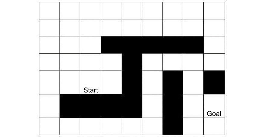
Figure 1.16: Shortest pathfinding game board
We import math and heapq:
import math
import heapq
Next, we'll reuse the initialization code from Steps 2–5 of the previous, Exercise 1.05, Finding the Shortest Path Using BFS.
Note
We have omitted the function to update costs because we will do so within the A* algorithm:
Next, we need to initialize the A* algorithm's frontier and internal lists. For frontier, we will use a Python PriorityQueue. Do not execute this code directly; we will use these four lines inside the A* search function:
frontier = []
internal = set()
heapq.heappush(frontier, (0, start))
costs = initialize_costs(size, start)
Now, it is time to implement a heuristic function that measures the distance between the current node and the goal node using the algorithm we saw in the heuristic section:
def distance_heuristic(node, goal):
    (x, y) = node
    (u, v) = goal
    return math.sqrt(abs(x - u) ** 2 + abs(y - v) ** 2)
The final step will be to translate the A* algorithm into functioning code:
def astar(start, end):
    frontier = []
    internal = set()
    heapq.heappush(frontier, (0, start))
    costs = initialize_costs(size, start)
    def get_distance_from_start(node):
       return costs[node[0] - 1][node[1] - 1]
    def set_distance_from_start(node, new_distance):
        costs[node[0] - 1][node[1] - 1] = new_distance
    while len(frontier) > 0:
        (priority, node) = heapq.heappop(frontier)
        if node == end:
            return priority
        internal.add(node)
        successor_nodes = successors(node, internal)
        for s in successor_nodes:
            new_distance = get_distance_from_start(node) + 1
            if new_distance < get_distance_from_start(s):
                set_distance_from_start(s, new_distance)
                # Filter previous entries of s
                frontier = [n for n in frontier if s != n[1]]
                heapq.heappush(frontier, \
                              (new_distance \
                              + distance_heuristic(s, end), s))
astar(start, end)
The expected output is this:
15.0
There are a few differences between our implementation and the original algorithm.
We defined a distance_from_start function to make it easier and more semantic to access the costs matrix. Note that we number the node indices starting with 1, while in the matrix, indices start with zero. Therefore, we subtract 1 from the node values to get the indices.
When generating the successor nodes, we automatically ruled out nodes that are in the internal set. successors = succ(node, internal) makes sure that we only get the neighbors whose examination is not closed yet, meaning that their score is not necessarily optimal.
Therefore, we may skip the step check since internal nodes will never end up in succ(n).
Since we are using a priority queue, we must determine the estimated priority of nodes before inserting them. However, we will only insert the node in the frontier if we know that this node does not have an entry with a lower score.
It may happen that nodes are already in the frontier queue with a higher score. In this case, we remove this entry before inserting it into the right place in the priority queue. When we find the end node, we simply return the length of the shortest path instead of the path itself.
To follow what the A* algorithm does, execute the following example code and observe the logs:
def astar_verbose(start, end):
    frontier = []
    internal = set()
    heapq.heappush(frontier, (0, start))
    costs = initialize_costs(size, start)
    def get_distance_from_start(node):
        return costs[node[0] - 1][node[1] - 1]
    def set_distance_from_start(node, new_distance):
        costs[node[0] - 1][node[1] - 1] = new_distance
    steps = 0
    while len(frontier) > 0:
        steps += 1
        print('step ', steps, '. frontier: ', frontier)
        (priority, node) = heapq.heappop(frontier)
        print('node ', node, \
              'has been popped from frontier with priority', \
              priority)
        if node == end:
            print('Optimal path found. Steps: ', steps)
            print('Costs matrix: ', costs)
            return priority
        internal.add(node)
        successor_nodes = successors(node, internal)
        print('successor_nodes', successor_nodes)
        for s in successor_nodes:
            new_distance = get_distance_from_start(node) + 1
            print('s:', s, 'new distance:', new_distance, \
                  ' old distance:', get_distance_from_start(s))
            if new_distance < get_distance_from_start(s):
                set_distance_from_start(s, new_distance)
                # Filter previous entries of s
                frontier = [n for n in frontier if s != n[1]]
                new_priority = new_distance \
                               + distance_heuristic(s, end)
                heapq.heappush(frontier, (new_priority, s))
                print('Node', s, \
                      'has been pushed to frontier with priority', \
                      new_priority)
    print('Frontier', frontier)
    print('Internal', internal)
    print(costs)
astar_verbose(start, end)
Here, we build the astar_verbose function by reusing the code from the astar function and adding print functions in order to create a log.
The expected output is this:
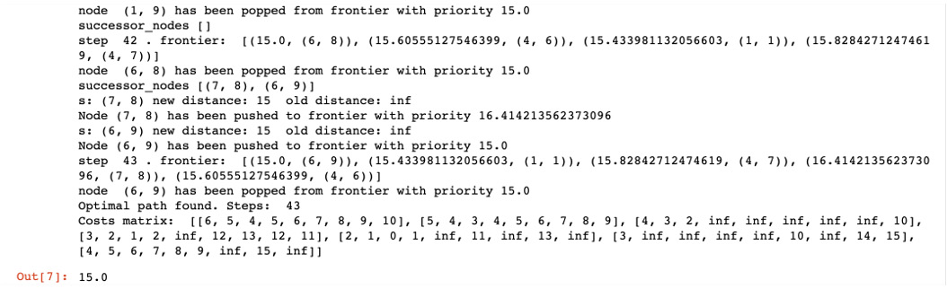
Figure 1.17: Astar function logs
We have seen that the A* search returns the right values. The question is, how can we reconstruct the whole path?
For this, we remove the print statements from the code for clarity and continue with the A* algorithm that we implemented in the previous step. Instead of returning the length of the shortest path, we have to return the path itself. We will write a function that extracts this path by walking backward from the end node, analyzing the costs matrix. Do not define this function globally yet. We define it as a local function in the A* algorithm that we created previously:
def get_shortest_path(end_node):
    path = [end_node]
    distance = get_distance_from_start(end_node)
    while distance > 0:
        for neighbor in successors(path[-1], []):
            new_distance = get_distance_from_start(neighbor)
            if new_distance < distance:
                path += [neighbor]
                distance = new_distance
                break  # for
    return path
Now that we've seen how to deconstruct the path, let's return it inside the A* algorithm:
def astar_with_path(start, end):
    frontier = []
    internal = set()
    heapq.heappush(frontier, (0, start))
    costs = initialize_costs(size, start)
    def get_distance_from_start(node):
        return costs[node[0] - 1][node[1] - 1]
    def set_distance_from_start(node, new_distance):
        costs[node[0] - 1][node[1] - 1] = new_distance
    def get_shortest_path(end_node):
        path = [end_node]
        distance = get_distance_from_start(end_node)
        while distance > 0:
            for neighbor in successors(path[-1], []):
                new_distance = get_distance_from_start(neighbor)
                if new_distance < distance:
                    path += [neighbor]
                    distance = new_distance
                    break  # for
        return path
    while len(frontier) > 0:
        (priority, node) = heapq.heappop(frontier)
        if node == end:
            return get_shortest_path(end)
        internal.add(node)
        successor_nodes = successors(node, internal)
        for s in successor_nodes:
            new_distance = get_distance_from_start(node) + 1
            if new_distance < get_distance_from_start(s):
                set_distance_from_start(s, new_distance)
                # Filter previous entries of s
                frontier = [n for n in frontier if s != n[1]]
                heapq.heappush(frontier, \
                              (new_distance \
                              + distance_heuristic(s, end), s))
astar_with_path( start, end )
In the preceding code snippet, we have reused the a-star function defined previously with the notable difference of adding the get_shortest_path function. Then, we use this function to replace the priority queue since we want the algorithm to always choose the shortest path.
The expected output is this:
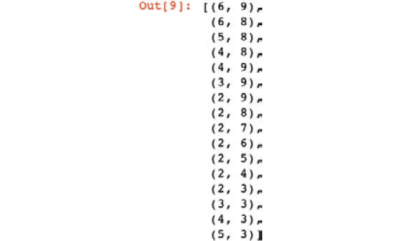
Figure 1.18: Output showing the priority queue
Technically, we do not need to reconstruct the path from the costs matrix. We could record the parent node of each node in the matrix and simply retrieve the coordinates to save a bit of searching.
We are not expecting you to understand all the preceding script as it is quite advanced, so we are going to use a library that will simplify it for us.
A* Search in Practice Using the simpleai Library
The simpleai library is available on GitHub and contains many popular AI tools and techniques.
Note
You can access this library at https://github.com/simpleai-team/simpleai. The documentation of the simpleai library can be accessed here: http://simpleai.readthedocs.io/en/latest/. To access the simpleai library, first, you have to install it.
The simpleai library can be installed as follows:
pip install simpleai
Once simpleai has been installed, you can import classes and functions from the simpleai library into a Jupyter Notebook:
from simpleai.search import SearchProblem, astar
SearchProblem gives you a frame for defining any search problems. The astar import is responsible for executing the A* algorithm inside the search problem.
For simplicity, we have not used classes in the previous code examples to focus on the algorithms in a plain old style without any clutter.
Note
Remember that the simpleai library will force us to use classes.
To describe a search problem, you need to provide the following:
constructor: This initializes the state space, thus describing the problem. We will make theSize,Start,End, andObstaclesvalues available in the object by adding it to these as properties. At the end of the constructor, do not forget to call the super constructor, and do not forget to supply the initial state.actions( state ): This returns a list of actions that we can perform from a given state. We will use this function to generate new states. Semantically, it would make more sense to create action constants such as UP, DOWN, LEFT, and RIGHT, and then interpret these action constants as a result. However, in this implementation, we will simply interpret an action as "move to(x, y)", and represent this command as(x, y). This function contains more-or-less the logic that we implemented in thesuccfunction previously, except that we won't filter the result based on a set of visited nodes.result( state0, action): This returns the new state of action that was applied tostate0.is_goal( state ): This returnstrueif the state is a goal state. In our implementation, we will have to compare the state to the end state coordinates.cost( self, state, action, newState ): This is the cost of moving fromstatetonewStateviaaction. In our example, the cost of a move is uniformly 1.
Have a look at the following example:
import math
from simpleai.search import SearchProblem, astar
class ShortestPath(SearchProblem):
    def __init__(self, size, start, end, obstacles):
        self.size = size
        self.start = start
        self.end = end
        self.obstacles = obstacles
        super(ShortestPath, \
              self).__init__(initial_state=self.start)
    def actions(self, state):
        (row, col) = state
        (max_row, max_col) = self.size
        succ_states = []
        if row > 1:
            succ_states += [(row-1, col)]
        if col > 1:
            succ_states += [(row, col-1)]
        if row < max_row:
            succ_states += [(row+1, col)]
        if col < max_col:
            succ_states += [(row, col+1)]
        return [s for s in succ_states \
                if s not in self.obstacles]
    def result(self, state, action):
        return action
    def is_goal(self, state):
        return state == end
    def cost(self, state, action, new_state):
        return 1
    def heuristic(self, state):
        (x, y) = state
        (u, v) = self.end
        return math.sqrt(abs(x-u) ** 2 + abs(y-v) ** 2)
size = (7, 9)
start = (5, 3)
end = (6, 9)
obstacles = {(3, 4), (3, 5), (3, 6), (3, 7), (3, 8), \
             (4, 5), (5, 5), (5, 7), (5, 9), (6, 2), \
             (6, 3), (6, 4), (6, 5), (6, 7), (7, 7)}
searchProblem = ShortestPath(size, start, end, obstacles)
result = astar(searchProblem, graph_search=True)
result.path()
In the preceding code snippet, we used the simpleai package to simplify our code. We also had to define a class called ShortestPath in order to use the package.
The expected output is this:
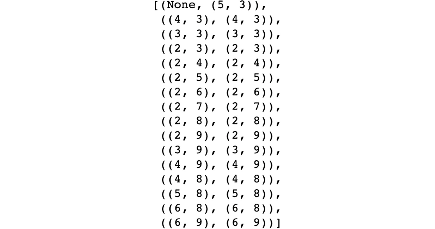
Figure 1.19: Output showing the queue using the simpleai library
The simpleai library made the search description a lot easier than the manual implementation. All we need to do is define a few basic methods, and then we have access to an effective search implementation.
In the next section, we will be looking at the Minmax algorithm, along with pruning.