All the magic in this model lies behind the RNN cells. In our simple example, each cell presents the same equations, just with a different set of variables. A detailed version of a single cell looks like this:
First, let's explain the new terms that appear in the preceding diagram:
- Weights (
 ,
,  ,
,  ): A weight is a matrix (or a number) that represents the strength of the value it is applied to. For example,
  determines how much of the input
  should be considered in the following equations.
If  consists of high values, then
  should have significant influence on the end result. The weight values are often initialized randomly or with a distribution (such as normal/Gaussian distribution). It is important to be noted that
  ,
,  , and
, and  are the same for each step. Using the backpropagation algorithm, they are being modified with the aim of producing accurate predictions
- Biases (
 ,
,  ): An offset vector (different for each layer), which adds a change to the value of the output
- Activation function (tanh): This determines the final value of the current memory state
 and the output
  . Basically, the activation functions map the resultant values of several equations similar to the following ones into a desired range: (-1, 1) if we are using the tanh function, (0, 1) if we are using sigmoid function, and (0, +infinity) if we are using ReLu (https://ai.stackexchange.com/questions/5493/what-is-the-purpose-of-an-activation-function-in-neural-networks)
Now, let's go over the process of computing the variables. To calculate  and , we can do the following:
As you can see, the memory state  is a result of the previous value
  and the input
  . Using this formula helps in retaining information about all the previous states.
The input  is a one-hot representation of the word volunteer. Recall from before that one-hot encoding is a type of word embedding. If the text corpus consists of 20,000 unique words and volunteer is the 19th word, then
  is a 20,000-dimensional vector where all elements are 0 except the one at the 19th position, which has a value of 1, which suggests that we only taking into account this particular word.
The sum between  ,
,  , and
, and  is passed to the tanh activation function, which squashes the result between -1 and 1 using the following formula:
In this, e = 2.71828 (Euler's number) and z is any real number.
The output  at time step t is calculated using
  and the softmax function. This function can be categorized as an activation with the exception that its primary usage is at the output layer when a probability distribution is needed. For example, predicting the correct outcome in a classification problem can be achieved by picking the highest probable value from a vector where all the elements sum up to 1. Softmax produces this vector, as follows:
In this, e = 2.71828 (Euler's number) and z is a K-dimensional vector. The formula calculates probability for the value at the ith position in the vector z.
After applying the softmax function,  becomes a vector of the same dimension as
  (the corpus size 20,000) with all its elements having a total sum of 1. With that in mind, finding the predicted word from the text corpus becomes straightforward.


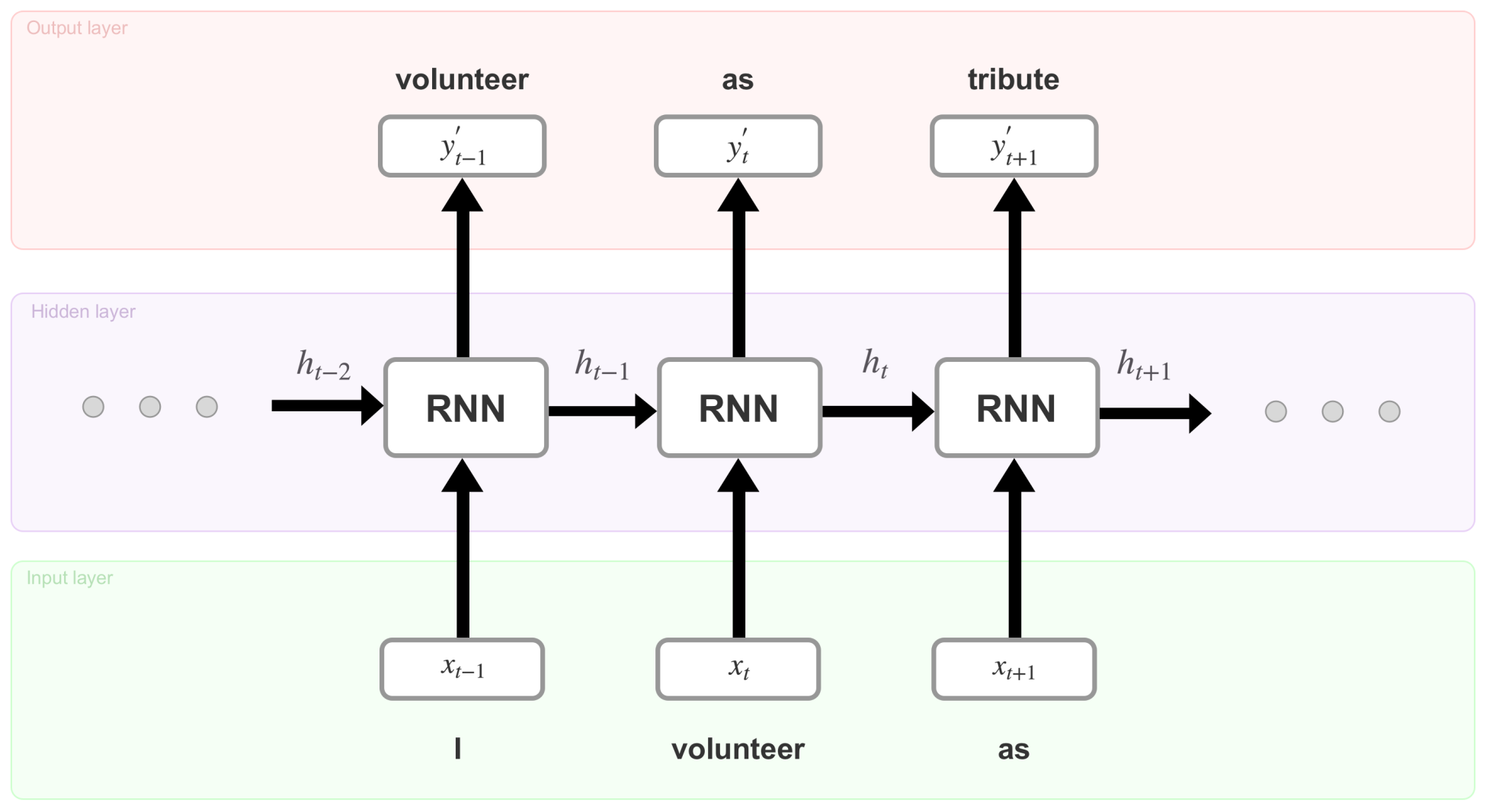
 + RNN +
  illustrates what is happening at time step
  . At each time step, these operations perform as follows:
 (The produced vector can be
  or
or  depending on the specific time step)
 , the encoded version of the input word I at time step t-1, is plugged into the RNN cell (located in the hidden layer). After several equations (not displayed here but happening inside the RNN cell), the cell produces an output
  and a memory state
  . The memory state is the result of the input
  and the previous value of that memory state
  . For the initial time step, one can assume that
  is a zero vector
 ,
,  ,
,  , …} holds information about all the previous inputs. This makes RNNs very special and really good at predicting the next unit in a sequence. Let's now see what mathematical equations sit behind the preceding operations.
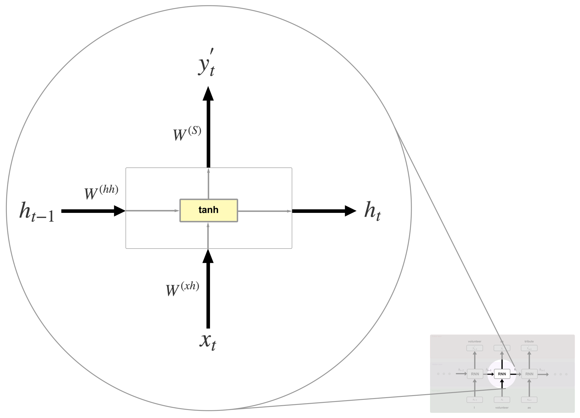


 with the actual word from the training data (let's call it
  ). This operation can be accomplished using a loss (cost) function. These types of functions aim to find the error between predicted and actual values. Our choice will be the cross-entropy loss function, which looks like this: