Search icon
Arrow left icon
All Products
Best Sellers
New Releases
Books
Videos
Audiobooks
Learning Hub
Newsletters
Free Learning
Arrow right icon
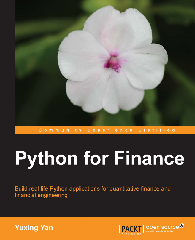
Python for Finance

You're reading from  Python for Finance

Product type Book
Published in Apr 2014
Publisher
ISBN-13 9781783284375
Pages 408 pages
Edition 1st Edition
Languages
Author (1):
Yuxing Yan Yuxing Yan
Profile icon Yuxing Yan

Table of Contents (20) Chapters

Python for Finance
Credits
About the Author
Acknowledgments
About the Reviewers
www.PacktPub.com
Preface
Introduction and Installation of Python Using Python as an Ordinary Calculator Using Python as a Financial Calculator 13 Lines of Python to Price a Call Option Introduction to Modules Introduction to NumPy and SciPy Visual Finance via Matplotlib Statistical Analysis of Time Series The Black-Scholes-Merton Option Model Python Loops and Implied Volatility Monte Carlo Simulation and Options Volatility Measures and GARCH Index

Chapter 12. Volatility Measures and GARCH

In finance, we know that risk is defined as uncertainty since we are unable to predict the future more accurately. Based on the assumption that prices follow a lognormal distribution and returns follow a normal distribution, we could define risk as standard deviation or variance of the returns of a security. We call this our conventional definition of volatility (uncertainty). Since a normal distribution is symmetric, it will treat a positive deviation from a mean in the same manner as it would a negative deviation. This is against our conventional wisdom since we treat them differently. To overcome this, Sortino (1983) suggests a lower partial standard deviation. Up to now, we assume that the volatility of a time series is a constant. Obviously this is not true. Another observation is volatility clustering, which means that high volatility is usually followed by a high-volatility period, and this is true for low volatility that is usually followed...

Conventional volatility measure – standard deviation


In most finance textbooks, we use the standard deviation of returns as a risk measure. This is based on a critical assumption that log returns follow a normal distribution. Even both standard deviation and variance could be used to measure uncertainty; the former is usually called volatility itself. For example, if we say that the volatility of IBM is 20 percent, it means that its annualized standard deviation is 20 percent. Using IBM as an example, the following program is used to estimate its annualized volatility:

from matplotlib.finance import quotes_historical_yahoo
import numpy as np
ticker='IBM'
begdate=(2009,1,1)
enddate=(2013,12,31)
p = quotes_historical_yahoo(ticker, begdate, enddate,asobject=True, adjusted=True)
ret = (p.aclose[1:] - p.aclose[:-1])/p.aclose[1:]
std_annual=np.std(ret)*np.sqrt(252)

From the following output, we know that the volatility is 20.87 percent for IBM:

>>>print 'volatility (std)=',round(std_annual...

Tests of normality


The Shapiro-Wilk test is a normality test. The following Python program verifies whether IBM's returns are following a normal distribution. The last five-year daily data from Yahoo! Finance is used for the test. The null hypothesis is that IBM's daily returns are drawn from a normal distribution:

from scipy import stats
from matplotlib.finance import quotes_historical_yahoo
import numpy as np
ticker='IBM'
begdate=(2009,1,1)
enddate=(2013,12,31)
p = quotes_historical_yahoo(ticker, begdate, enddate,asobject=True, adjusted=True)
ret = (p.aclose[1:] - p.aclose[:-1])/p.aclose[1:]
print 'ticker=',ticker,'W-test, and P-value'
print stats.shapiro(ret)

The results are shown as follows:

The first value of the result is the test statistic, and the second one is its corresponding p-value. Since this p-value is so close to zero, we reject the null hypothesis. In other words, we conclude that IBM's daily returns do not follow a normal distribution.

For the normality test, we could also...

Lower partial standard deviation


One issue with using standard deviation of returns as a risk measure is that the positive deviation is also viewed as bad. The second issue is that the deviation is from the average instead of a fixed benchmark, such as a risk-free rate. To overcome these shortcomings, Sortino (1983) suggests the lower partial standard deviation, which is defined as the average of squared deviation from the risk-free rate conditional on negative excess returns, as shown in the following formula:

Because we need the risk-free rate in this equation, we could generate a Fama-French dataset that includes the risk-free rate as one of their time series. First, download their daily factors from http://mba.tuck.dartmouth.edu/pages/faculty/ken.french/data_library.html.Then, unzip it and delete the non-data part at the end of the text file. Assume the final text file is saved under C:/temp/:

import pandas as pd
import datetime
file=open("c:/temp/F-F_Research_Data_Factors_daily.txt"...

Test of equivalency of volatility over two periods


We know that the stock market fell dramatically in October, 1987. We could choose a stock to test the volatility before and after October, 1987. For instance, we could use Ford Motor Corp, with a ticker of F, to illustrate how to test the equality of variance before and after the market crash in 1987. In the following Python program, we define a function called ret_f() to retrieve daily price data from Yahoo! Finance and estimate its daily returns:

import scipy as sp
from matplotlib.finance import quotes_historical_yahoo
import numpy as np
# input area 
ticker='F'               # stock
begdate1=(1982,9,1)      # starting date for period  #1
enddate1=(1987,9,1)      # ending   date for period  #1
begdate2=(1987,12,1)     # starting date for period  #2
enddate2=(1992,12,1)     # ending   date for period  #2
# define a function
def ret_f(ticker,begdate,enddate):
    p = quotes_historical_yahoo(ticker, begdate, enddate,asobject=True, adjusted...

Test of heteroskedasticity, Breusch, and Pagan (1979)


Breusch and Pagan (1979) designed a test to confirm or reject the null assumption that the residuals from a regression is homogeneous, that is, with a constant volatility. The following formula represents their logic. First, we run a linear regression of y against x:

Here, y is the independent variable, x is the independent variable, α is the intercept, β is the coefficient and is an error term. After we get the error term (residual), we run the second regression:

Assume that the fitted values from running the previous regression is , then the Breusch-Pangan (1979) measure is given as follows, and it follows a χ2 distribution with a k degree of freedom:

The following example is borrowed from an R package called lm.test (test linear regression), and its authors are Hothorn et al. (2014). We generate a time series of x, y1 and y2. The independent variable is x, and the dependent variables are y1 and y2. By our design, y1 is homogeneous,...

Retrieving option data from Yahoo! Finance


In the previous chapter, we discussed in detail how to estimate implied volatility with a hypothetic set of input values. To use real-world data to estimate implied volatility, we could define a function with three input variables: ticker, month, and year as follows:

def get_option_data(tickrr,exp_date):
    x = Options(ticker,'yahoo')
    puts,calls = x.get_options_data(expiry=exp_date)
    return puts, calls

To call the function, we enter three values, such as IBM, 2, and 2014, when we plan to retrieve options expired in February, 2014. The code with these three values is shown as follows:

def from pandas.io.data import Options
import datetime
ticker='IBM'
exp_date=datetime.date(2014,2,28)
puts, calls =get_option_data(ticker,exp_date)
print puts.head()
Strike              Symbol  Last  Chg   Bid   Ask  Vol  Open Int
0     100  IBM140222P00100000  0.01    0   NaN  0.03   16        16
1     105  IBM140222P00105000  0.04    0   NaN  0.03   10   ...

Volatility smile and skewness


Obviously, each stock should possess just one volatility. However, when estimating implied volatility, different strike prices might offer us different implied volatilities. More specifically, the implied volatility based on out-of-the-money options, at-the-money options, and in-the-money options might be quite different. Volatility smile is the shape going down then up with the exercise prices, while the volatility skewness is downward or upward sloping. The key is that investors' sentiments and the supply and demand relationship have a fundamental impact on the volatility skewness. Thus, such a smile or skewness provides information on whether investors such as fund managers prefer to write calls or puts, as shown in the following code:

from pandas.io.data import Options
from matplotlib.finance import quotes_historical_yahoo
# Step 1: define two functions 
def call_data(tickrr,exp_date):
    x = Options(ticker,'yahoo')
    data= x.get_call_data(expiry=exp_date...

The ARCH model


Based on previous arguments, we know that the volatility or variance of stock returns is not constant. According to the ARCH model, we could use the error terms from pervious estimation to help us predict the next volatility or variance. This model was developed by Robert F. Engle, the winner of the 2003 Nobel Prize in Economics. The formula for an ARCH (q) model is presented as follows:

Here, is the variance at time t, is the ith coefficient, is the squared error term for the period of t-I, and q is the order of error terms. When q is 1, we have the simplest ARCH (1) process as follows:

Simulating an ARCH (1) process

It is a good idea that we simulate an ARCH (1) process and have a better understanding of the volatility clustering, which means that high volatility is usually followed by a high-volatility period while low volatility is usually followed by a low-volatility period. The following code reflects this phenomenon:

import scipy as sp
sp.random.seed(12345)
n=1000 ...

The GARCH (Generalized ARCH) model


Generalized AutoRegressive Conditional Heteroskedasticity (GARCH) is an important extension of ARCH, by Bollerslev (1986). The GARCH (p,q) process is defined as follows:

Here, is the variance at time t, q is the order for the error terms, p is the order for the variance, is a constant, is the coefficient for the error term at t-i, is the coefficient for the variance at time t-i. Obviously, the simplest GARCH process is when both p and q are set to 1, that is, GARCH (1,1), which has following formula:

Simulating a GARCH process

Based on the previous program related to ARCH (1), we could simulate a GARCH (1,1) process as follows:

import scipy as sp
sp.random.seed(12345)
n=1000          # n is the number of observations
n1=100          # we need to drop the first several observations
n2=n+n1         # sum of two numbers
alpha=(0.1,0.3)     # GARCH (1,1) coefficients alpha0 and alpha1, see Equation (3)
beta=0.2
errors=sp.random.normal(0,1,n2)
t=sp.zeros(n2...

Summary


In this chapter, we focused on several issues, especially on volatility measures and ARCH/GARCH. For the volatility measures, first we discussed the widely used standard deviation, which is based on the normality assumption. To show that such an assumption might not hold, we introduced several normality tests, such as the Shapiro-Wilk test and the Anderson-Darling test. To show a fat tail of many stocks' real distribution benchmarked on a normal distribution, we vividly used various graphs to illustrate it. To show that the volatility might not be constant, we presented the test to compare the variance over two periods. Then, we showed a Python program to conduct the Breusch-Pangan (1979) test for heteroskedasticity. ARCH and GARCH are used widely to describe the evolvements of volatility over time. For these models, we simulate their simple form such as ARCH (1) and GARCH (1,1) processes. In addition to their graphical presentations, the Python codes of Kevin Sheppard are included...

Exercises


1. What is the definition of volatility?

2. How can you measure risk (volatility)?/

3. What are the issues related to the widely used definition of risk (standard deviation)?

4. How can you test whether stock returns follow a normal distribution? For given sets of stocks, test whether they follow a normal distribution.

5. What is the lower partial standard deviation? What are its applications?

6. Choose five stocks, such as DELL, IBM, Microsoft, Citi Group, and Walmart, and compare their standard deviation with LPSD based on the last three-years' daily data.

7. Is a stock's volatility constant over the years?

8. Use the Breusch-Pagan (1979) test to confirm or reject the hypothesis that daily returns for IBM is homogeneous.

9. How can you test whether a stock's volatility is constant?

10. What does "fat tail" mean ? Why should we care about fat tail?

11. How can you download the option data?

12. What is an ARCH (1) process?

13. What is a GARCH (1,1) process?

14. Apply GARCH (1,1) process to...

lock icon The rest of the chapter is locked
You have been reading a chapter from
Python for Finance
Published in: Apr 2014 Publisher: ISBN-13: 9781783284375
Register for a free Packt account to unlock a world of extra content!
A free Packt account unlocks extra newsletters, articles, discounted offers, and much more. Start advancing your knowledge today.
Unlock this book and the full library FREE for 7 days
Get unlimited access to 7000+ expert-authored eBooks and videos courses covering every tech area you can think of
Renews at $15.99/month. Cancel anytime}