Search icon
Arrow left icon
All Products
Best Sellers
New Releases
Books
Videos
Audiobooks
Learning Hub
Newsletters
Free Learning
Arrow right icon
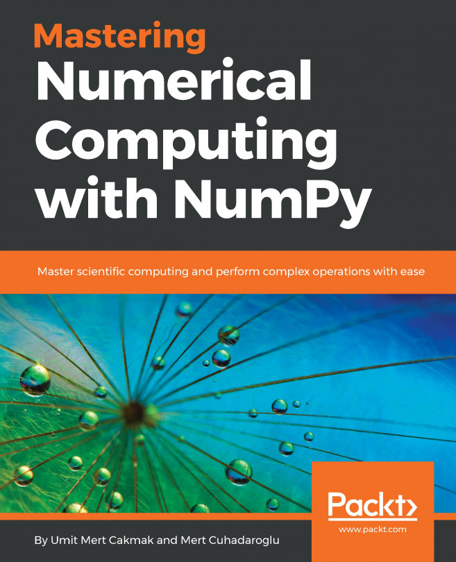
Mastering Numerical Computing with NumPy

You're reading from  Mastering Numerical Computing with NumPy

Product type Book
Published in Jun 2018
Publisher Packt
ISBN-13 9781788993357
Pages 248 pages
Edition 1st Edition
Languages
Authors (3):
Umit Mert Cakmak Umit Mert Cakmak
Profile icon Umit Mert Cakmak
Tiago Antao Tiago Antao
Profile icon Tiago Antao
Mert Cuhadaroglu Mert Cuhadaroglu
Profile icon Mert Cuhadaroglu
View More author details

Table of Contents (11) Chapters

Preface Working with NumPy Arrays Linear Algebra with NumPy Exploratory Data Analysis of Boston Housing Data with NumPy Statistics Predicting Housing Prices Using Linear Regression Clustering Clients of a Wholesale Distributor Using NumPy NumPy, SciPy, Pandas, and Scikit-Learn Advanced Numpy Overview of High-Performance Numerical Computing Libraries Performance Benchmarks Other Books You May Enjoy

Linear Algebra with NumPy

One of the major divisions of mathematics is algebra, and linear algebra in particular, focuses on linear equations and mapping linear spaces, namely vector spaces. When we create a linear map between vector spaces, we are actually creating a data structure called a matrix. The main usage of linear algebra is to solve simultaneous linear equations, but it can also be used for approximations for non-linear systems. Imagine a complex model or system that you are trying to understand, think of it as a non-linear model. In such cases, you can reduce the complex, non-linear characteristics of the problem into simultaneous linear equations, and you can solve them with the help of linear algebra.

In computer science, linear algebra is heavily used in machine learning (ML) applications. In ML applications, you deal with high-dimensional arrays, which can easily...

Vector and matrix mathematics

In the previous chapter, you practiced introductory operations with vectors and matrices. In this section, you will practice more advanced vector and matrix operations that are heavily used in linear algebra. Let's remember the dot product perspective on matrix manipulation and how it can be done with different methods when you have 2-D arrays. The following code block shows alternative ways of performing dot product calculation:

In [1]: import numpy as np 
a = np.arange(12).reshape(3,2)
b = np.arange(15).reshape(2,5)
print(a)
print(b)
Out[1]:
[[ 0 1]
[ 2 3]
[ 4 5]]
[[ 0 1 2 3 4]
[ 5 6 7 8 9]
In [2]: np.dot(a,b)
Out[2]: array([[ 5, 6, 7, 8, 9],
[15, 20, 25, 30, 35],
[25, 34, 43, 52, 61]])
In [3]: np.matmul(a,b)
Out[3]: array([[ 5, 6, 7, 8, 9],
[15, 20, 25, 30...

What's an eigenvalue and how do we compute it?

An eigenvalue is a coefficient of an eigenvector. By definition, an eigenvector is a non zero vector that only changes by a scalar factor when linear transformation is applied. In general, when linear transformation is applied to a vector, its span (the line passing through its origin) is shifted, but some special vectors are not affected by these linear transformations and remain on their own span. These are what we call eigenvectors. The linear transformation affects them only by stretching or squishing them as you are multiplying this vector with a scalar. The value of this scalar is called the eigenvalue. Let's say we have a matrix A, which will be used in linear transformation. We can represent the eigenvalue and eigenvector in a mathematical statements as follows:

Here, is the eigenvector and denotes the eigenvalue...

Computing the norm and determinant

This subsection will introduce two important values in linear algebra, namely the norm and determinant. Briefly, the norm gives length of a vector. The most commonly used norm is the L2-norm, which is also known as the Euclidean norm. Formally, the Lp-norm of x is calculated as follows:

The L0-norm is actually the cardinality of a vector. You can calculate it by just counting the total number of non-zero elements. For example, the vector A =[2,5,9,0] contains three non-zero elements, therefore ||A||0 = 3. The following code block shows the same norm calculation with numpy:

In [24]: import numpy as np 
x = np.array([2,5,9,0])
np.linalg.norm(x,ord=0)
Out[24]: 3.0

In NumPy, you can calculate the norm of the vector with the use of the linalg.norm() method. The first parameter is the input array and the ord parameter is for order...

Solving linear equations

In this section, you will learn how to solve linear equations by using the linalg.solve() method. When you have a linear equation to solve, as in the form , in simple cases you can just calculate the inverse of A and then multiply it by B to get the solution, but when A has a high dimensionality, that makes it very hard computationally to calculate the inverse of A. Let's start with an example of three linear equations with three unknowns, as follows:

So, these equations can be formalized as follows with matrices:

Then, our problem is to solve . We can calculate the solution with a plain vanilla NumPy without using linalg.solve(). After inverting the A matrix, you will multiply with B in order to get results for x. In the following code block, we calculate the dot product for the inverse matrix of A and B in order to calculate :

In [44]: A =...

Computing gradient

When you have a linear line, you take the derivative so the derivative shows the slope of this line. Gradient is a generalization of the derivative when you have a multiple variable in your function, therefore the result of gradient is actually a vector function rather than a scalar value in derivative. The main goal of ML is actually finding the best model that fits your data. You can evaluate the meaning of the best as minimizing your loss function or objective function. Gradient is used for finding the value of the coefficients or a function that will minimize your loss or cost function. A well-known way of finding optimum points is taking the derivative of the objective function then setting it to zero to find your model coefficients. If you have more than one coefficient then it becomes a gradient rather than a derivative, and it becomes a vector equation...

Summary

In this chapter, we covered vector and matrix operations for linear algebra. We looked at advanced matrix operations, especially featuring dot operations. You also learned about eigenvalues and eigenvectors and then practiced their use in principal component analysis (PCA). Moreover, we covered the norm and determinant calculation and mentioned their importance and usage in ML. In the last two subsections, you learned how to convert linear equations into matrices and solve them, and looked at the computation and importance of gradients.

In the next chapter, we will use NumPy statistics to do explanatory data analysis to explore the 2015 United States Housing data.

lock icon The rest of the chapter is locked
You have been reading a chapter from
Mastering Numerical Computing with NumPy
Published in: Jun 2018 Publisher: Packt ISBN-13: 9781788993357
Register for a free Packt account to unlock a world of extra content!
A free Packt account unlocks extra newsletters, articles, discounted offers, and much more. Start advancing your knowledge today.
Unlock this book and the full library FREE for 7 days
Get unlimited access to 7000+ expert-authored eBooks and videos courses covering every tech area you can think of
Renews at $15.99/month. Cancel anytime}