


Machine learning is not traditional software
Although machine learning and artificial intelligence have been around since the 1950s, introduced by Alan Turing, they only became popular with the first MYCIN system and our understanding of machine learning systems changed over time. It was not until the 2010s that we started to perceive, design, and develop machine learning in the same way as we do today (in 2023). In my view, two pivotal moments shaped the landscape of machine learning as we see it today.
The first pivotal moment was the focus on big data in the late 2000s and early 2010s. With the introduction of smartphones, companies started to collect and process increasingly large quantities of data, mostly about our behavior online. One of the companies that perfected this was Google, which collected data about our searches, online behavior, and usage of Google’s operating system, Android. As the volume of the collected data increased (and its speed/velocity), so did its value and the need for its veracity – the five Vs. These five Vs – volume, velocity, value, veracity, and variety – required a new approach to working with data. The classical approach of relational databases (SQL) was no longer sufficient. Relational databases became too slow in handling high-velocity data streams, which gave way to map-reduce algorithms, distributed databases, and in-memory databases. The classical approach of relational schemas became too constraining for the variety of data, which gave way for non-SQL databases, which stored documents.
The second pivotal moment was the rise of modern machine learning algorithms – deep learning. Deep learning algorithms are designed to handle unstructured data such as text, images, or music (compared to structured data in the form of tables and matrices). Classical machine learning algorithms, such as regression, decision trees, or random forest, require data in a tabular form. Each row is a data point, and each column is one characteristic of it – a feature. The classical models are designed to handle relatively small datasets. Deep learning algorithms, on the other hand, can handle large datasets and find more complex patterns in the data because of the power of large neural networks and their complex architectures.
Machine learning is sometimes called statistical learning as it is based on statistical methods. The statistical methods calculate properties of data (such as mean values, standard deviations, and coefficients) and thus find patterns in the data. The core characteristic of machine learning is that it uses data to find patterns, learn from them, and then repeat these patterns on new data. We call this way of learning patterns training, and repeating these patterns as reasoning, or in machine learning language, predicting. The main benefits of using machine learning software come from the fact that we do not need to design the algorithms – we focus on the problem to be solved and the data that we use to solve the problem. Figure 1.1 shows an example of how such a flowchart of machine learning software can be realized.
First, we import a generic machine learning model from a library. This generic model has all elements that are specific to it, but it is not trained to solve any tasks. An example of such a model is a decision tree model, which is designed to learn dependencies in data in the form of decisions (or data splits), which it uses later for new data. To make this model somewhat useful, we need to train it. For that, we need data, which we call the training data.
Second, we evaluate the trained model on new data, which we call the test data. The evaluation process uses the trained model and applies it to check whether its inferences are correct. To be precise, it checks to which degree the inferences are correct. The training data is in the same format as the test data, but the content of these datasets is different. No data point should be present in both.
In the third step, we use the model as part of a software system. We develop other non-machine learning components, and we connect them to the trained model. The entire software system usually consists of data procurement components, real-time validation components, data cleaning components, user interfaces, and business logic components. All these components, including the machine learning model, provide a specific functionality for the end user. Once the software system has been developed, it needs to be tested, which is where the input data comes into play. The input data is something that the end user inputs to the system, such as by filling in a form. The input data is designed in such a way that has both the input and expected output – to test whether the software system works correctly.
Finally, the last step is to deploy the entire system. The deployment can be very different, but most modern machine learning systems are organized into two parts – the onboard/edge algorithms for non-machine learning components and the user interface, and the offboard/cloud algorithms for machine learning inferences. Although it is possible to deploy all parts of the system on the target device (both machine learning and non-machine learning components), complex machine learning models require significant computational power for good performance and seamless user experience. The principle is simple – more data/complex data means more complex models, which means that more computational power is needed:
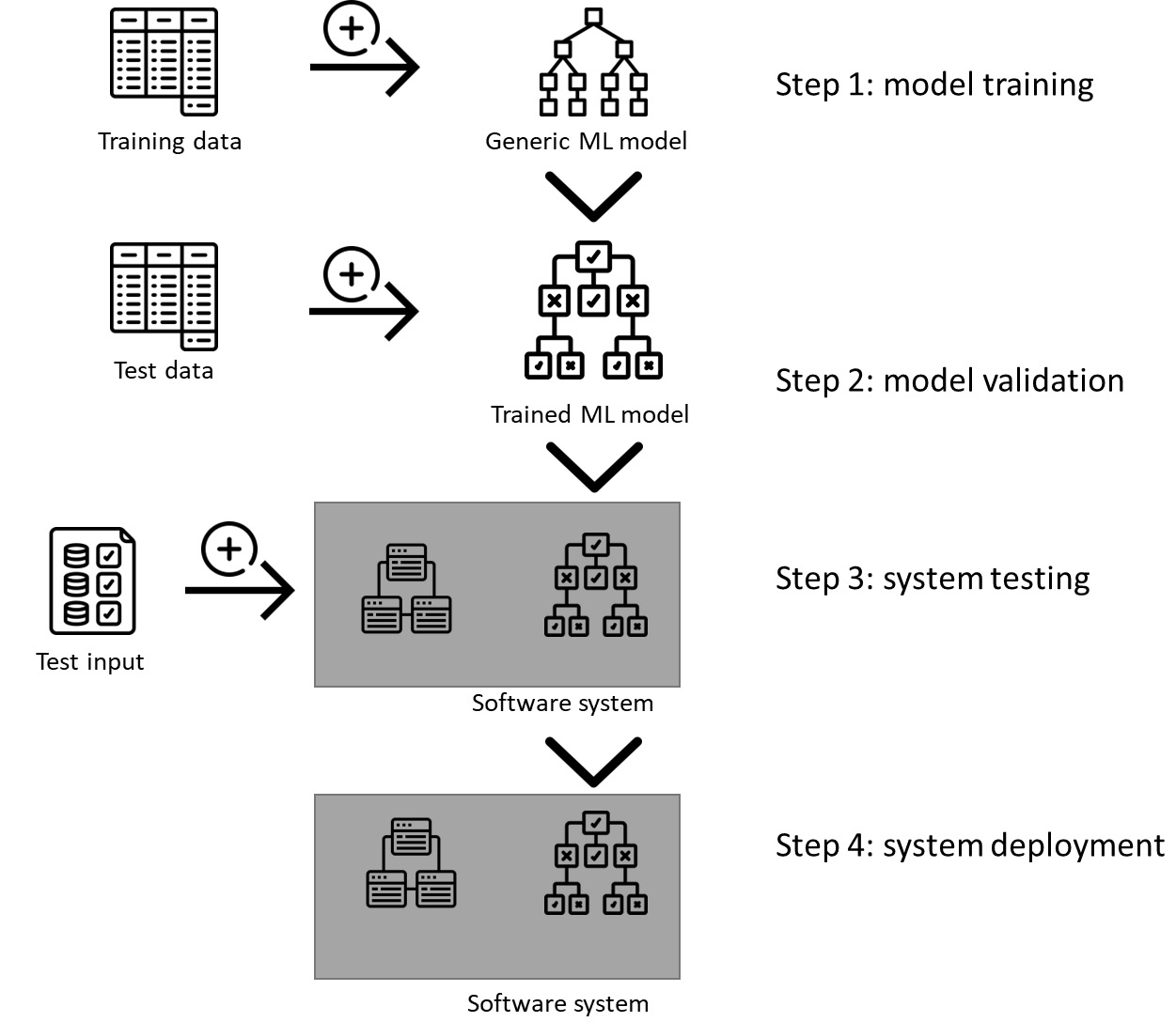
Figure 1.1 – Typical flow of machine learning software development
As shown in Figure 1.1, one of the crucial elements of the machine learning software is the model, which is one of the generic machine learning models, such as a neural network, that’s been trained on specific data. Such a model is used to make predictions and inferences. In most systems, this kind of component – the model – is often prototyped and developed in Python.
Models are trained for different datasets and, therefore, the core characteristic of machine learning software is its dependence on that dataset. An example of such a model is a vision system, where we train a machine learning algorithm such as a convolutional neural network (CNN) to classify images of cats and dogs.
Since the models are trained on specific datasets, they perform best on similar datasets when making inferences. For example, if we train a model to recognize cats and dogs in 160 x 160-pixel grayscale images, the model can recognize cats and dogs in such images. However, the same model will perform very poorly (if at all!) if it needs to recognize cats and dogs in colorful images instead of grayscale images – the accuracy of the classification will be low (close to 0).
On the other hand, when we develop and design traditional software systems, we do not rely on data that much, as shown in Figure 1.2. This figure provides an overview of a software development process for traditional, non-machine learning software. Although it is depicted as a flow, it is usually an iterative process where Steps 1 to 3 are done in cycles, each one ending with new functionality added to the product.
The first step is developing the software system. This includes the development of all its components – user interface, business logic (processing), handling of data, and communication. The step does not involve much data unless the software engineer creates data for testing purposes.
The second step is system testing, where we use input data to validate the software system. In essence, this step is almost identical to testing machine learning software. The input data is complemented with the expected outcome data, which allows software testers to assess whether the software works correctly.
The third step is to deploy the software. The deployment can be done in many ways. However, if we consider traditional software that is similar in function to machine learning software, it is usually simpler. It usually does not require deployment on the cloud, just like machine learning models:
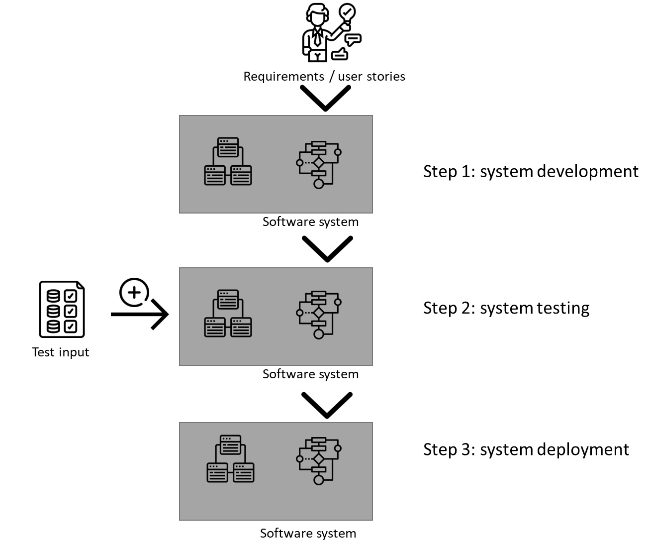
Figure 1.2 - Typical flow of traditional software development
The main difference between traditional software and machine learning-based software is that we need to design, develop, and test all the elements of the traditional software. In machine learning-based software, we take an empty model, which contains all the necessary elements, and we use the data to train it. We do not need to develop the individual components of the machine learning model from scratch.
One of the main parts of traditional software is the algorithm, which is developed by software engineers from scratch, based on the requirements or user stories. The algorithm is usually written as a sequential set of steps that are implemented in a programming language. Naturally, all algorithms use data to operate on it, but they do it differently than machine learning systems. They do it based on the software engineer’s design – if x, then y or something similar.
We usually consider these traditional algorithms as deterministic, explainable, and traceable. This means that the software engineer’s design decisions are documented in the algorithm and the algorithm can be analyzed afterward. They are deterministic because they are programmed based on rules; there is no training from data or identifying patterns from data. They are explainable because they are designed by programmers and each line of the program has a predefined meaning. Finally, they are traceable as we can debug every step of these programs.
However, there is a drawback – the software engineer needs to thoroughly consider all corner cases and understand the problem very well. The data that the software engineer uses is only to support them in analyzing the algorithm, not training it.
An example of a system that can be implemented using both machine learning algorithms and traditional ones is one for reading passport information. Instead of using machine learning for image recognition, the software uses specific marks in the passport (usually the <<< sequence of characters) to mark the beginning of the line or the beginning of the sequence of characters denoting a surname. These marks can be recognized quite quickly using rule-based optical character recognition (OCR) algorithms without the need for deep learning or CNNs.
Therefore, I would like to introduce the first best practice.
Best practice #1
Use machine learning algorithms when your problem is focused on data, not on the algorithm.
When selecting the right technology, we need to understand whether it is based on the classical approach, where the design of the algorithm is in focus, or whether we need to focus on handling data and finding patterns in it. It is usually beneficial to start with the following guidelines.
If the problem requires processing large quantities of data in raw format, use the machine learning approach. Examples of such systems are conversational bots, image recognition tools, text processing tools, or even prediction systems.
However, if the problem requires traceability and control, use the traditional approach. Examples of such systems are control software in cars (anti-lock braking, engine control, and so on) and embedded systems.
If the problem requires new data to be generated based on the existing data, a process known as data manipulation, use the machine learning approach. Examples of such systems are image manipulation programs (DALL-E), text generation programs, deep fake programs, and source code generation programs (GitHub Copilot).
If the problem requires adaptation over time and optimization, use machine learning software. Examples of such systems are power grid optimization software, non-playable character behavior components in computer games, playlist recommendation systems, and even GPS navigation systems in modern cars.
However, if the problem requires stability and traceability, use the traditional approach. Examples of such systems are systems to make diagnoses and recommendation systems in medicine, safety-critical systems in cars, planes, and trains, and infrastructure controlling and monitoring systems.
Supervised, unsupervised, and reinforcement learning – it is just the beginning
Now is a good time to mention that the field of machine learning is huge, and it is organized into three main areas – supervised learning, unsupervised learning, and reinforcement learning. Each of these areas has hundreds of different algorithms. For example, the area of supervised learning has over 1,000 algorithms, all of which can be automatically selected by meta-heuristic algorithms such as AutoML:
- Supervised learning: This is a group of algorithms that are trained based on annotated data. The data that’s used in these algorithms needs to have a target or a label. The label is used to tell the algorithm which pattern to look for. For example, such a label can be cat or dog for each image that the supervised learning model needs to recognize. Historically, supervised learning algorithms are the oldest ones as they come directly from statistical methods such as linear regression and multinomial regression. Modern algorithms are advanced and include methods such as deep learning neural networks, which can recognize objects in 3D images and segment them accordingly. The most advanced algorithms in this area are deep learning and multimodal models, which can process text and images at the same time.
A sub-group of supervised learning algorithms is self-supervised models, which are often based on transformer architectures. These models do not require labels in the data, but they use the data itself as labels. The most prominent examples of these algorithms are translation models for natural languages and generative models for images or texts. Such algorithms are trained by masking words in the original texts and predicting them. For the generative models, these algorithms are trained by masking parts of their output to predict it.
- Unsupervised learning: This is a group of models that are applied to find patterns in data without any labels. These models are not trained, but they use statistical properties of the input data to find patterns. Examples of such algorithms are clustering algorithms and semantic map algorithms. The input data for these algorithms is not labeled and the goal of applying these algorithms is to find structure in the dataset according to similarities; these structures can then be used to add labels to this data. We encounter these algorithms daily when we get recommendations for products to buy, books to read, music to listen to, or films to watch.
- Reinforcement learning: This is a group of models that are applied to data to solve a particular task given a goal. For these models, we need to provide this goal in addition to the data. It is called the reward function, and it is an expression that defines when we achieve the goal. The model is trained based on this fitness function. Examples of such models are algorithms that play Go, Chess, or StarCraft. These algorithms are also used to solve hard programming problems (AlphaCode) or optimize energy consumption.
So, let me introduce the second best practice.
Best practice #2
Before you start developing a machine learning system, do due diligence and identify the right group of algorithms to use.
As each of these groups of models has different characteristics, solves different problems, and requires different data, a mistake in selecting the right algorithm can be costly. Supervised models are very good at solving problems related to predictions and classifications. The most powerful models in this area can compete with humans in selected areas – for example, GitHub Copilot can create programs that can pass as human-written. Unsupervised models are very powerful if we want to group entities and make recommendations. Finally, reinforcement learning models are the best when we want to have continuous optimization with the need to retrain models every time the data or the environment changes.
Although all these models are based on statistical learning, they are all components of larger systems to make them useful. Therefore, we need to understand how this probabilistic and statistical nature of machine learning goes with traditional, digital software products.
An example of traditional and machine learning software
To illustrate the difference between traditional software and machine learning software, let’s implement the same program using these two paradigms. We’ll implement a program that calculates a Fibonacci sequence using the traditional approach, which we have seen a million times in computer science courses. Then, we’ll implement the same program using machine learning models – or one model to be exact – that is, logistic regression.
The traditional implementation is presented here. It is based on one recursive function and a loop that tests it:
# a recursive function to calculate the fibonacci number
# this is a standard solution that is used in almost all
# of computer science examples
def fibRec(n):
  if n < 2:
      return n
  else:
      return fibRec(n-1) + fibRec(n-2)
# a short loop that uses the above function
for i in range(23):
  print(fibRec(i))
The implementation is very simple and is based on the algorithm – in our case, the fibRec function. It is simplistic, but it has its limitations. The first one is its recursive implementation, which costs resources. Although it can be written as an iterative one, it still suffers from the second problem – it is focused on the calculations and not on the data.
Now, let’s see how the machine learning implementation is done. I’ll explain this by dividing it into two parts – data preparation and model training/inference:
#predicting fibonacci with linear regression
import pandas as pd
import numpy as np
from sklearn.linear_model import LinearRegression
# training data for the algorithm
# the first two columns are the numbers and the third column is the result
dfTrain = pd.DataFrame([[1, 1, 2],
                        [2, 1, 3],
                        [3, 2, 5],
                        [5, 3, 8],
                        [8, 5, 13]
])
# now, let's make some predictions
# we start the sequence as a list with the first two numbers
lstSequence = [0,1]
# we add the names of the columns to make it look better
dfTrain.columns = ['first number','second number','result']
In the case of machine learning software, we prepare data to train the algorithm. In our case, this is the dfTrain DataFrame. It is a table that contains the numbers that the machine learning algorithm needs to find the pattern.
Please note that we prepared two datasets – dfTrain, which contains the numbers to train the algorithm, and lstSequence, which is the sequence of Fibonacci numbers that we’ll find later.
Now, let’s start training the algorithm:
# algorithm to train
# here, we use linear regression
model = LinearRegression()
# now, the actual process of training the model
model.fit(dfTrain[['first number', 'second number']],
                               dfTrain['result'])
# printing the score of the model, i.e. how good the model is when trained
print(model.score(dfTrain[['first number', 'second number']], dfTrain['result']))
The magic of the entire code fragment is in the bold-faced code – the model.fit method call. This method trains the logistic regression model based on the data we prepared for it. The model itself is created one line above, in the model = LinearRegression() line.
Now, we can make inferences or create new Fibonacci numbers using the following code fragment:
# and loop through the newly predicted numbers
for k in range(23):
  # the line below is where the magic happens
  # it takes two numbers from the list
  # formats them to an array
  # and makes the prediction
  # since the model returns a float,
  # we need to convert it to it
  intFibonacci = int(model.predict(np.array([[lstSequence[k],lstSequence[k+1]]])))
  # add this new number to the list for the next iteration
  lstSequence.append(intFibonacci)
  # and print it
  print(intFibonacci)
This code fragment contains a similar line to the previous one – model.predict(). This line uses the previously created model to make an inference. Since the Fibonacci sequence is recursive, we need to add the newly created number to the list before we can make the new inference, which is done in the lstSequence.append() line.
Now, it is very important to emphasize the difference between these two ways of solving the same problem. The traditional implementation exposes the algorithm used to create the numbers. We do not see the Fibonacci sequence there, but we can see how it is calculated. The machine learning implementation exposes the data used to create the numbers. We see the first sequence as training data, but we never see how the model creates that sequence. We do not know whether that model is always correct – we would need to test it against the real sequence – simply because we do not know how the algorithm works. This takes us to the next part, which is about just that – probabilities.