Chapter 2. Image Filtering

In the previous chapter, we started off on our journey into the world of computer vision and image processing by familiarizing ourselves with some terms that occur frequently when we talk about images. We also had our first contact with OpenCV when we learnt about how the library provides us with efficient data structures to store and process image data. The chapter also helped us get acquainted with some basic algorithms within the realm of image processing by expounding the details of linear and logarithmic transformations. We familiarized ourselves with how these enhancement techniques essentially work to improve the image contrast (hence the name image enhancement), and saw them in action as they modified (stretched or compressed) the grayscale range of an image, thereby revealing details hidden in the darker and lighter regions of the image.

This chapter will take our journey forward. We will learn about more techniques that act on images, perform certain forms...

Neighborhood of a pixel

We have seen image processing operations where the value of a pixel at the output is dependent only on the value of the corresponding pixel at the input. By corresponding, we mean pixels at the same locations (row and column) in the input and output image. Such transformations were represented in mathematical form as follows:

s = T(r)

Here, s and r are the intensity values of a pixel in the output and input respectively. Since we are always dealing with pixels at the same locations, there is no mention of pixel coordinates in the preceding formula. That is to say, the grayscale value of the pixel at the 40^th row and 30th column in the output depends on the grayscale value of the pixel at the same coordinates (the 40^th row and 30^th column) at the input.

This section will introduce you to a slightly more advanced form of image transformation. In the operations that we'll discuss now, the output value at a particular pixel (x, y) is not only dependent on the intensity...

Image averaging

Now that we are familiar with the notion of a neighborhood, we are ready to delve into the details of an operation called image averaging. As the name suggests, image averaging involves taking the mean of pixel intensity values. More specifically, each pixel is replaced by the mean of all pixels in its neighborhood. The size of the neighborhood is one of the parameters that is usually passed to the function that implements this sort of an averaging procedure. For illustration purposes, we consider a neighborhood of 3 x 3 around the pixel (this would include the pixel and its eight immediate neighbors). For example, consider the next image (you can take it to be a small sub-section within the entire image). Let's say that we wish to compute the output intensity value corresponding to the pixel with an intensity of 6 in the input image. We take the 3 x 3 neighborhood of that pixel and calculate the mean of all those values (the values have been marked in bold-face). Hence,...

Image filters

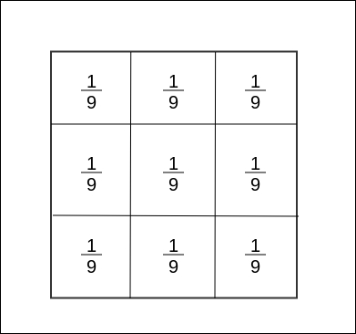
If you carefully observe the example that we discussed in the previous section, you will notice that during the process of computing the output intensity at (x, y), we basically multiplied the intensity values of all the 3 x 3 neighbors by 1/9 and added them all up. Let's create a small matrix of dimensions 3 x 3 (the size of the neighborhood under consideration) and fill all the cells with the value 1/9 as shown in the following image:

We'll call this a filter or a kernel. Now, we'll make use of this filter to calculate the output intensity value corresponding to any arbitrary input pixel (x, y), say the pixel having an intensity value of 6 (see the following image). How do we go about doing that? Well, we place the filter over the image in such a manner that the central grid in the filter lies right on top of the pixel at position (x, y)-(2, 2) in our case (I have assumed 1-based indexing for both rows and columns). Once we place the filter in this manner, it will completely...

Image averaging in OpenCV

While implementing the image transforms that we discussed in the previous chapter, we adopted an approach that was based on the fundamentals and involved quite a bit of reinventing the wheel. We could afford to do that because the traversals that we performed over the data matrix in our implementations were conceptually pretty straightforward. However, we will no longer do that for a couple of reasons:

• The kind of transformations that we are discussing at the moment (averaging using a filtering-based approach) no longer involves a simple pixel-by-pixel traversal of the data matrix. Rather, they involve a two-tiered approach where we have to traverse the neighborhood for each pixel that we encounter in our usual traversal of the data matrix. Implementing such a non-trivial traversal every single time can become time-consuming and error-prone.

• As we progress through the book, we want you to rely more and more on the functions and APIs provided by the OpenCV developers...

Blurring an image in OpenCV

Since we are already familiar with the basics, let's jump right into the code. I am skipping the header declarations because they remain the same as we saw in our previous code:

int main() 
{ 
  Mat input_image = imread("lena.png", IMREAD_GRAYSCALE); 
  Mat filtered_image; 
  blur(input_image, filtered_image, Size(3, 3), Point(-1, -1), BORDER_REPLICATE); 
   
  imshow("Original Image", input_image); 
  imshow("Filtered Image", filtered_image); 
  waitKey(0); 
  return 0; 
} 

The first thing that you notice about the blur() function is that the number of arguments is less than its counterpart. Upon a closer inspection, you'll find that the following two arguments are missing:

• Depth of the output image: According to OpenCV's documentation for blur(), the output image has the same size and type as the source image. Since the equality between the input and output image types is already enforced by the implementation...

Gaussian smoothing

In the image smoothing operation that we introduced in the last section, we used a 3 x 3 filter where every value was 1/9. When we discussed the working of a filter, we explained that every element in a filter multiplies itself with the intensity value of a pixel in the neighborhood and the result is added up (this was one way to visualize the averaging operation). Now, we will present one more technique to visualize the same!

I am guessing that you are aware of the concept of weighted averages. For those who are not, we reiterate the same here. Given a sequence of n values and their corresponding weights , the weighted average of these n values is given by the following relation:

In the special case where all of the weights sum up to 1, our equation reduces to the following:

This form is starting to feel a little familiar now, isn't it? What if the weights  correspond to the values in our filter and the sequence  is our pixel intensity values? Well, in that case the...

Gaussian function and Gaussian filtering

Very shortly, we will be embarking on a long, but rather interesting discussion as we build our mathematical intuitions on Gaussian filtering. In order to motivate the same, we present to you some sample images that have been generated by applying the Gaussian filtering operation on Lena's image. A detailed description of each of the succeeding four output images will be presented at the end of this section. Right now, this is to motivate you and give you a glimpse of what to expect as we move ahead!

For the purpose of explaining the theoretical underpinnings and working of the Gaussian filtering method, we take a step back and consider 1D images. Just as regular 2D images are represented using a 2D grid of values, in the same manner (hypothetical) 1D images are nothing but a 1D array of pixel values.

The preceding diagram attempts to visualize the workings of a simple 1x3 box filter that replaces each pixel with the average of itself and its immediate...

Gaussian filtering in OpenCV

We have spent a considerable amount of time understanding the theory behind Gaussian filtering. It is now time to jump into the implementation. The headers will remain the same as in the case of boxFilter(). The functions implementing Gaussian filtering also reside within the imgproc module:

#include <iostream> 
#include <opencv2/core/core.hpp> 
#include <opencv2/highgui/highgui.hpp> 
#include <opencv2/imgproc/imgproc.hpp> 
 
using namespace std; 
using namespace cv; 

Here is the code snippet that actually accomplishes the task of Gaussian filtering:

int main() { 
    Mat input_image = imread("lena.jpg", IMREAD_GRAYSCALE); 
    Mat filtered_image; 
 
    GaussianBlur(input_image, filtered_image, Size(7, 7), 1.0, 1.0, BORDER_REPLICATE); 
 
    imshow("Filtered Image", filtered_image); 
    waitKey(0); 
    return 0; 
} 

One of the first things that you probably...

Using your own filters in OpenCV

So far, we have talked about a couple of different filtering techniques: box filtering and Gaussian filtering. Both of them had their own set of rules for defining a filter and also had a dedicated set of functions to help you apply the filters to images. When we introduced the concept of filtering, we said that different operations can be performed on our images by simply changing the value of the filter. So, if we design our own custom filter, how do we apply that to our image? There needs to exist a function that is more generic than boxFilter(), blur(), or GaussianBlur() and that will help us in applying the filter that we have designed to our input image. And OpenCV has the answer for you--the filter2D() function.

We have already hinted at what the filter2D() hopes to accomplish, so let's jump right into the code! I think at this point, I really don't need to say what the first few lines should look like:

#include <iostream> 
#include <opencv2...

Image noise

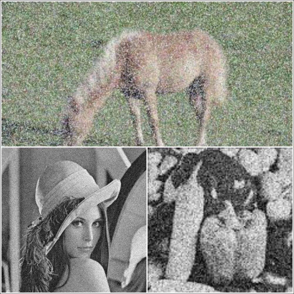
We have learnt in great detail about image filtering operations (box and Gaussian filtering). We have also seen that, in general, image averaging tends to blur our input image. Let us now stop and ponder why (and in what scenario) we would need to perform such averaging operations. What prompted the need to replace each pixel with an average (or a weighted average of its neighbors)? The answer to these questions lies in the concept of image noise.

Images are nothing but two-dimensional signals (mapping a pair of x and y coordinate values to corresponding pixel intensities) and just like any signal, they are susceptible to noise. When we say that an image is noisy, we mean that there is a small or large variation in the intensity values of the pixels from the ideal value that we would expect. Noise in an image creeps in due to defects in digital cameras or photographic film.

The following image demonstrates some examples of noisy photographs:

There are two different types of noise...

Vignetting

So far, we have introduced the concept of image filtering and discussed a couple of important filtering techniques, namely box filtering and Gaussian filtering. We also implemented the same using OpenCV and demonstrated the blurring effects that it produced on images. You can now experiment with the extent or degree of blurring by playing around with the size (and the standard deviation in the case of Gaussian filtering) of the image filters.

In this section, we are going to do something even more exciting! We are going to implement a basic version of a very cool image editing technique called Vignetting. For those of you who have come across this term in the context of popular image processing apps (such as Instagram), you will have seen it being referred to as the Vignetting filter or Vignette filter. However, since we are computer vision enthusiasts, we know that the term filter holds a very special meaning in our literature. Hence, we refrain from using the term filter for...

Implementing Vignetting in OpenCV

Now that you know about the type of changes that a Vignette mask brings about in images, we can start to think about devising a strategy for the same and ultimately go about implementing the Vignetting operation. As we have discussed, the Vignette mask leaves the central portion of an image bright and darkens the borders in all directions as we move out of the center. Now, the input image (grayscale) that we will be dealing with will have a fixed intensity value for every pixel. What we essentially need to do is modify the value of every pixel in such a manner that the pixels in the center remain at their original intensity levels while the surrounding pixels get progressively darker as we approach the borders.

How can we bring about such a transformation? Well, one way to do that would be to multiply each pixel value with a scaling constant between 0 and 1. The pixels whose intensities need to be kept as is (the ones near the center of the image) should...

Summary

In this chapter, we have continued our journey from the previous one. Filtering operations have been the primary focus of our study. The chapter started off by describing an image averaging operation and then went on to explain how such an operation may be conceptualized by visualizing the same in terms of filters. We then continued to generalize our concept of filters by demonstrating the basics of how any form of filtering is performed on images. By now, you must have realized that we are no longer dealing with simple pixel transformations similar to the ones that we discussed in the last chapter (grayscale transformations). When we talk of filtering operations, the computations at each pixel become much more sophisticated and involve a neighborhood around the pixel.

We learnt about a couple of different filtering techniques: box filtering and Gaussian filtering. Box filtering assumes an equal contribution from all the neighboring pixels in computing the weighted average. This assumption...