


Preparations
We will find the code for this example here: https://github.com/PacktPublishing/Interpretable-Machine-Learning-with-Python-2E/tree/main/02/CVD.ipynb.
Loading the libraries
To run this example, we need to install the following libraries:
mldatasetsto load the datasetpandasandnumpyto manipulate itstatsmodelsto fit the logistic regression modelsklearn(scikit-learn) to split the datamatplotlibandseabornto visualize the interpretations
We should load all of them first:
import math
import mldatasets
import pandas as pd
import numpy as np
import statsmodels.api as sm
from sklearn.model_selection import train_test_split
import matplotlib.pyplot as plt
import seaborn as sns
Understanding and preparing the data
The data to be used in this example should then be loaded into a DataFrame we call cvd_df:
cvd_df = mldatasets.load("cardiovascular-disease")
From this, we should get 70,000 records and 12 columns. We can take a peek at what was loaded with info():
cvd_df.info()
The preceding command will output the names of each column with its type and how many non-null records it contains:
RangeIndex: 70000 entries, 0 to 69999
Data columns (total 12 columns):
age            70000 non-null int64
gender         70000 non-null int64
height         70000 non-null int64
weight         70000 non-null float64
ap_hi          70000 non-null int64
ap_lo          70000 non-null int64
cholesterol    70000 non-null int64
gluc           70000 non-null int64
smoke          70000 non-null int64
alco           70000 non-null int64
active         70000 non-null int64
cardio         70000 non-null int64
dtypes: float64(1), int64(11)
The data dictionary
To understand what was loaded, the following is the data dictionary, as described in the source:
age: Of the patient in days (objective feature)height: In centimeters (objective feature)weight: In kg (objective feature)gender: A binary where 1: female, 2: male (objective feature)ap_hi: Systolic blood pressure, which is the arterial pressure exerted when blood is ejected during ventricular contraction. Normal value: < 120 mmHg (objective feature)ap_lo: Diastolic blood pressure, which is the arterial pressure in between heartbeats. Normal value: < 80 mmHg (objective feature)cholesterol: An ordinal where 1: normal, 2: above normal, and 3: well above normal (objective feature)gluc: An ordinal where 1: normal, 2: above normal, and 3: well above normal (objective feature)smoke: A binary where 0: non-smoker and 1: smoker (subjective feature)alco: A binary where 0: non-drinker and 1: drinker (subjective feature)active: A binary where 0: non-active and 1: active (subjective feature)cardio: A binary where 0: no CVD and 1: has CVD (objective and target feature)
It’s essential to understand the data generation process of a dataset, which is why the features are split into two categories:
- Objective: A feature that is a product of official documents or a clinical examination. It is expected to have a rather insignificant margin of error due to clerical or machine errors.
- Subjective: Reported by the patient and not verified (or unverifiable). In this case, due to lapses of memory, differences in understanding, or dishonesty, it is expected to be less reliable than objective features.
At the end of the day, trusting the model is often about trusting the data used to train it, so how much patients lie about smoking can make a difference.
Data preparation
For the sake of interpretability and model performance, there are several data preparation tasks that we can perform, but the one that stands out right now is age. Age is not something we usually measure in days. In fact, for health-related predictions like this one, we might even want to bucket them into age groups since health differences observed between individual year-of-birth cohorts aren’t as evident as those observed between generational cohorts, especially when cross tabulating with other features like lifestyle differences. For now, we will convert all ages into years:
cvd_df['age'] = cvd_df['age'] / 365.24
The result is a more understandable column because we expect age values to be between 0 and 120. We took existing data and transformed it. This is an example of feature engineering, which is when we use the domain knowledge of our data to create features that better represent our problem, thereby improving our models. We will discuss this further in Chapter 11, Bias Mitigation and Causal Inference Methods. There’s value in performing feature engineering simply to make model outcomes more interpretable as long as this doesn’t significantly hurt model performance. In fact, it might improve predictive performance. Note that there was no loss in data in the feature engineering performed on the age column, as the decimal value for years is maintained.
Now we are going to take a peek at what the summary statistics are for each one of our features using the describe() method:
cvd_df.describe(percentiles=[.01,.99]).transpose()
Figure 2.1 shows the summary statistics outputted by the preceding code. It includes the 1% and 99% percentiles, which tell us what are among the highest and lowest values for each feature:
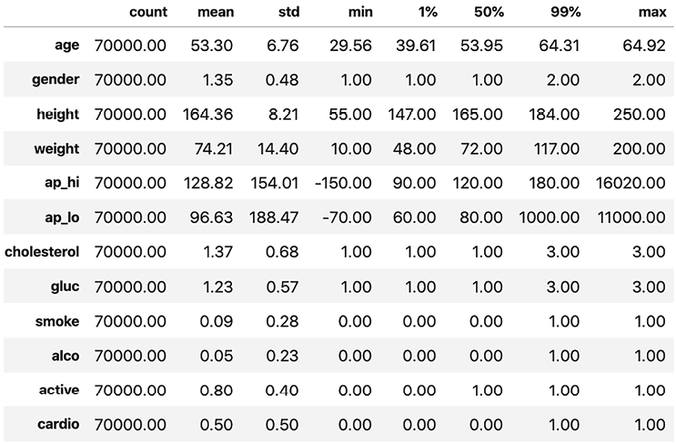
Figure 2.1: Summary statistics for the dataset
In Figure 2.1, age appears valid because it ranges between 29 and 65 years, which is not out of the ordinary, but there are some anomalous outliers for ap_hi and ap_lo. Blood pressure can’t be negative, and the highest ever recorded was 370. Keeping these outliers in there can lead to poor model performance and interpretability. Given that the 1% and 99% percentiles still show values in normal ranges according to Figure 2.1, there’s close to 2% of records with invalid values. If you dig deeper, you’ll realize it’s closer to 1.8%.
incorrect_l = cvd_df[
    (cvd_df['ap_hi']>370)
    | (cvd_df['ap_hi']<=40)
    | (cvd_df['ap_lo'] > 370)
    | (cvd_df['ap_lo'] <= 40)
].index
print(len(incorrect_l) / cvd_df.shape[0])
There are many ways we could handle these incorrect values, but because they are relatively few records and we lack the domain expertise to guess if they were mistyped (and correct them accordingly), we will delete them:
cvd_df.drop(incorrect_l, inplace=True)
For good measure, we ought to make sure that ap_hi is always higher than ap_lo, so any record with that discrepancy should also be dropped:
cvd_df = cvd_df[cvd_df['ap_hi'] >=\
                cvd_df['ap_lo']].reset_index(drop=True)
Now, in order to fit a logistic regression model, we must put all objective, examination, and subjective features together as X and the target feature alone as y. After this, we split X and y into training and test datasets, but make sure to include random_state for reproducibility:
y = cvd_df['cardio']
X = cvd_df.drop(['cardio'], axis=1).copy()
X_train, X_test, y_train, y_test = train_test_split(
    X, y, test_size=0.15, random_state=9
)
The scikit-learn train_test_split function puts 15% of the observations in the test dataset and the remainder in the train dataset, so you end up with X and y pairs for both.
Now that we have our data ready for training, let’s train a model and interpret it.


