Learning the terminology and physical memory layout

As mentioned before, the Arrow columnar format specification includes definitions of the in-memory data structures, metadata serialization, and protocols for data transportation. The format itself has a few key promises, as follows:

• Data adjacency for sequential access
• O(1) (constant time) random access
• SIMD and vectorization friendly
• Relocatable, allowing for zero-copy access in shared-memory

To ensure we're all on the same page, here's a quick glossary of terms that are used throughout the format specification and the rest of the book:

• Array: A list of values with a known length of the same type.
• Slot: The value in an array identified by a specific index.
• Buffer/contiguous memory region: A single contiguous block of memory with a given length.
• Physical layout: The underlying memory layout for an array without accounting for the interpretation of the logical value. For example, a 32-bit signed integer array and a 32-bit floating-point array are both laid out as contiguous chunks of memory where each value is made up of four contiguous bytes in the buffer.
• Parent/child arrays: Terms used for the relationship between physical arrays when describing the structure of a nested type. For example, a struct parent array has a child array for each of its fields.
• Primitive type: A type that has no child types and so consists of a single array, such as fixed-bit-width arrays (for example, int32) or variable-size types (for example, string arrays).
• Nested type: A type that depends on one or more other child types. Nested types are only equal if their child types are also equal (for example, List<T> and List<U> are equal if T and U are equal).
• Logical type: A particular type of interpreting the values in an array that is implemented using a specific physical layout. For example, the decimal logical type stores values as 16 bytes per value in a fixed-size binary layout. Similarly, a timestamp logical type stores values using a 64-bit fixed-size layout.

Now that we've got the fancy words out of the way, let's have a look at how we actually lay out these arrays in memory. An array or vector is defined by the following information:

• A logical data type (typically identified by an enum value and metadata)
• A group of buffers
• A length as a 64-bit signed integer
• A null count as a 64-bit signed integer
• Optionally, a dictionary for dictionary-encoded arrays (more on these later in the chapter)

To define a nested array type, there would additionally be one or more sets of this information that would then be the child arrays. Arrow defines a series of logical types and each one has a well-defined physical layout in the specification. For the most part, the physical layout just affects the sequence of buffers that make up the raw data. Since there is a null count in the metadata, it comes as a given that any value in an array may be considered to be null data rather than having a value, regardless of the type. Apart from the union data type, all the arrays have a validity bitmap as one of their buffers, which can optionally be left out if there are no nulls in the array. As might be expected, 1 in the corresponding bit means it is a valid value in that index, and 0 means it's null.

Quick summary of physical layouts, or TL;DR

When working with Arrow formatted data, it's important to understand how it is physically laid out in memory. Understanding the physical layouts can provide ideas for efficiently constructing (or deconstructing) Arrow data when developing applications. Here's a quick summary:

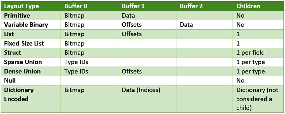
Figure 1.6 – Table of physical layouts

The following is a walkthrough of the physical memory layouts that are used by the Arrow format. This is primarily useful for either implementing the Arrow specification yourself (or contributing to the libraries) or if you simply want to know what's going on under the hood and how it all works.

Primitive fixed-length value arrays

Let's look at an example of a 32-bit integer array that looks like this: [1, null, 2, 4, 8]. What would the physical layout look like in memory based on the information so far (Figure 1.7)? Something to keep in mind is that all of the buffers should be padded to a multiple of 64 bytes for alignment, which matches the largest SIMD instructions available on widely deployed x86 architecture processors (Intel AVX-512), and that the values for null slots are marked UNF or undefined. Implementations are free to zero out the data in null slots if they desire, and many do. But, since the format specification does not define anything, the data in a null slot could technically be anything.

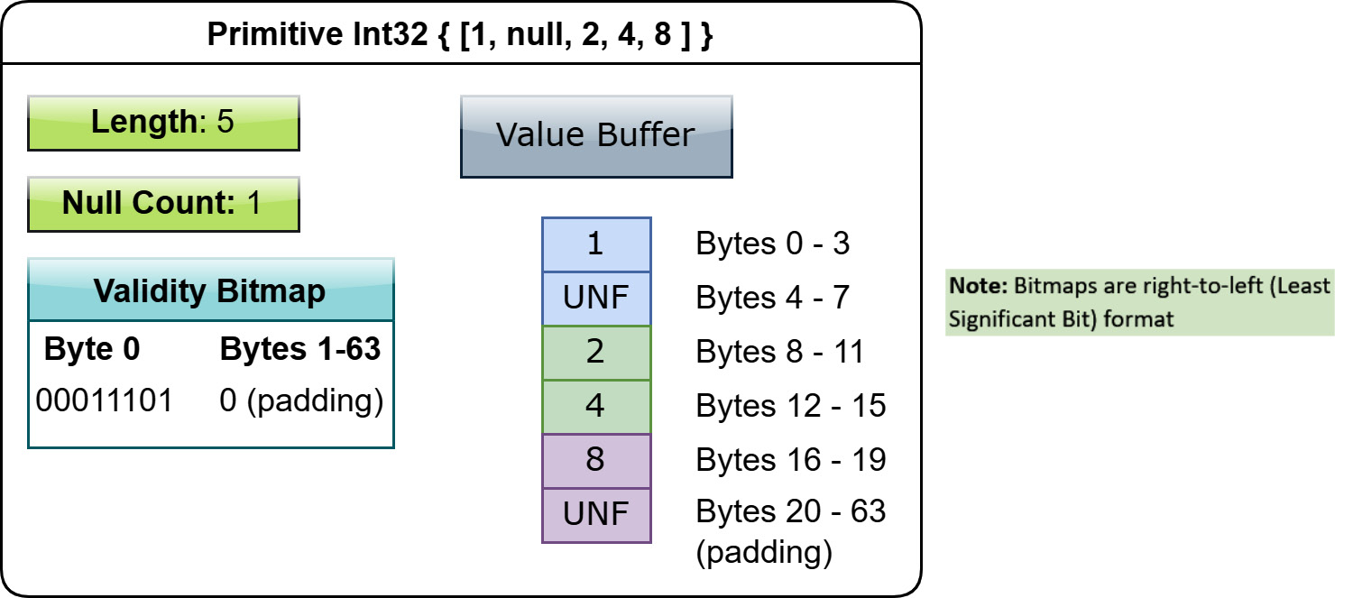
Figure 1.7 – Layout of primitive int32 array

This same conceptual layout is the case for any fixed-size primitive type, with the only exception being that the validity buffer can be left out entirely if there are no nulls in the array. For any data type that is physically represented as simple fixed-bit-width values, such as integers, floating-point values, fixed-size binary arrays, or even timestamps, it will use this layout in memory. The padding for the buffers in the subsequent diagrams will be left out just to avoid cluttering them.

Variable-length binary arrays

Things get slightly trickier when dealing with variable-length value arrays, generally used for variable size binary or string data. In this layout, every value can consist of 0 or more bytes and, in addition to the data buffer, there will also be an offsets buffer. Using an offsets buffer allows the entirety of the data of the array to be held in a single contiguous memory buffer. The only lookup cost for finding the value of a given index is to look up the indexes in the offsets buffer to find the correct slice of the data. The offsets buffer will always contain length + 1 signed integers (either 32-bit or 64-bit, based on the logical type being used) that indicate the starting position of each corresponding slot of the array. Consider the array of two strings: [ "Water", "Rising" ].

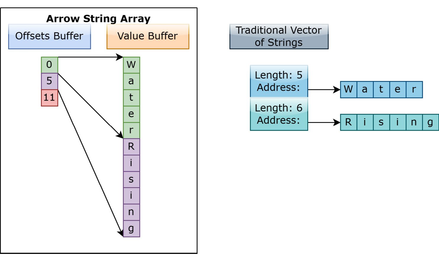
Figure 1.8 – Arrow string versus traditional string vector

This differs from a lot of standard ways of representing a list of strings in memory in most library models. Generally, a string is represented as a pointer to a memory location and an integer for the length, so a vector of strings is really a vector of these pointers and lengths (Figure 1.8). For many use cases, this is very efficient since, typically, a single memory address is going to be much smaller than the size of the string data, so passing around this address and length is efficient for referencing individual strings.

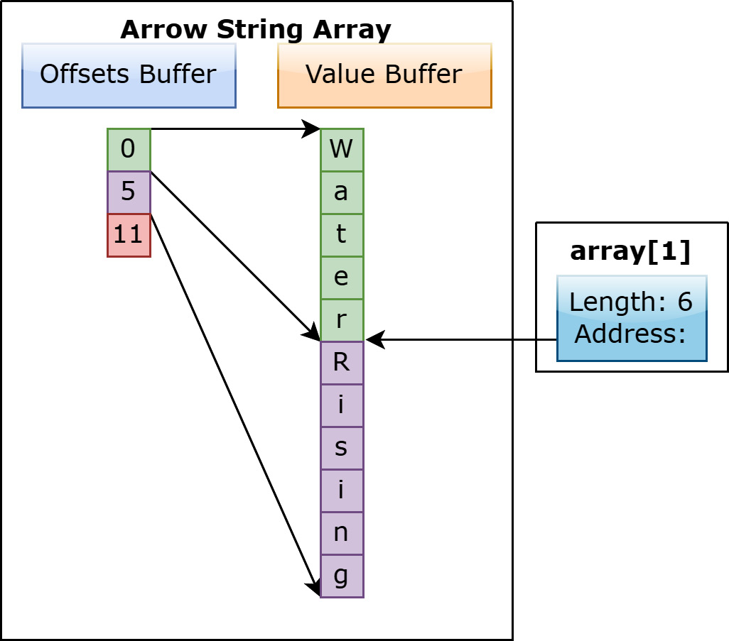
Figure 1.9 – Viewing string index 1

If your goal is operating on a large number of strings though, it's much more efficient to have a single buffer to scan through in memory. As you operate on each string, you can maintain the memory locality we mentioned before, keeping the memory we need to look at physically close to the next chunk of memory we're likely going to need. This way, we spend less time jumping around different pages of memory and can spend more CPU cycles performing the computations. It's also extremely efficient to get a single string, as you can simply take a view of the buffer by using the address indicated by the offset to create a string object without copying the data.

List and fixed-size list arrays

What about nested formats? Well, they work in a similar way to the variable-length binary format. First up is the variable-size list layout. It's defined by two buffers, a validity bitmap and an offsets buffer, along with a child array. The difference between this and the variable-length binary format is that instead of the offsets referencing a buffer, they are instead indexes into the child array (which could itself potentially be a nested type). The common denotation of list types is to specify them as List<T>, where T is any type at all. When using 64-bit offsets instead of 32-bit, it is denoted as LargeList<T>. Let's represent the following List<Int8> array: [[12, -7, 25], null, [0, -127, 127, 50], []].

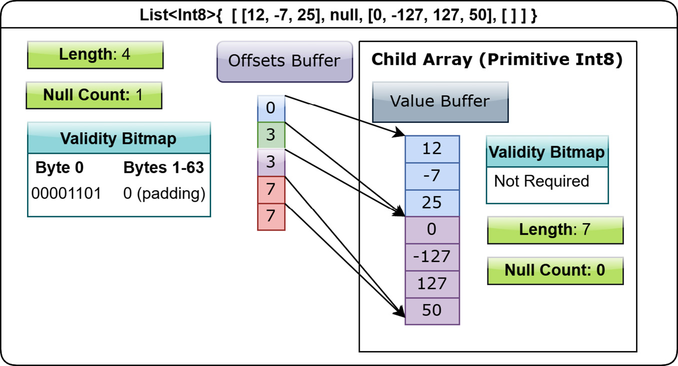
Figure 1.10 – Layout of list array

The first thing to notice in the preceding diagram is that the offsets buffer has exactly one more element than the List array it belongs to since there are four elements to our List<Int8> array and we have five elements in the offsets buffer. Each value in the offsets buffer represents the starting slot of the corresponding list index i. Looking closer at the offsets buffer, we notice that 3 and 7 are repeating, indicating that those lists are either null or empty (have a length of 0). To discover the length of a list at a given slot, you simply take the difference between the offset for that slot and the offset after it: , and the same holds true for the previous variable-length binary format; the number of bytes for a given slot is the difference in the offsets. Knowing this, what is the length of the list at index 2 of Figure 1.10? (remember, 0-based indexes!). With this, we can tell that the list at index 3 is empty because the bitmap has a 1, but the length is 0 (7 – 7). This also explains why we need that extra element in the offsets buffer! We need it to be able to calculate the length of the last element in the array.

Given that example, what would a List<List<Int8>> array look like? I'll leave that as an exercise for you to figure out.

There's also a FixedSizeList<T>[N] type, which works nearly the same as the variable-sized list, except there's no need for an offsets buffer. The child array of a fixed-size list type is the values array, complete with its own validity buffer. The value in slot of a fixed-size list array is stored in an -long slice of the values array, starting at offset . Figure 1.11 shows what this looks like:

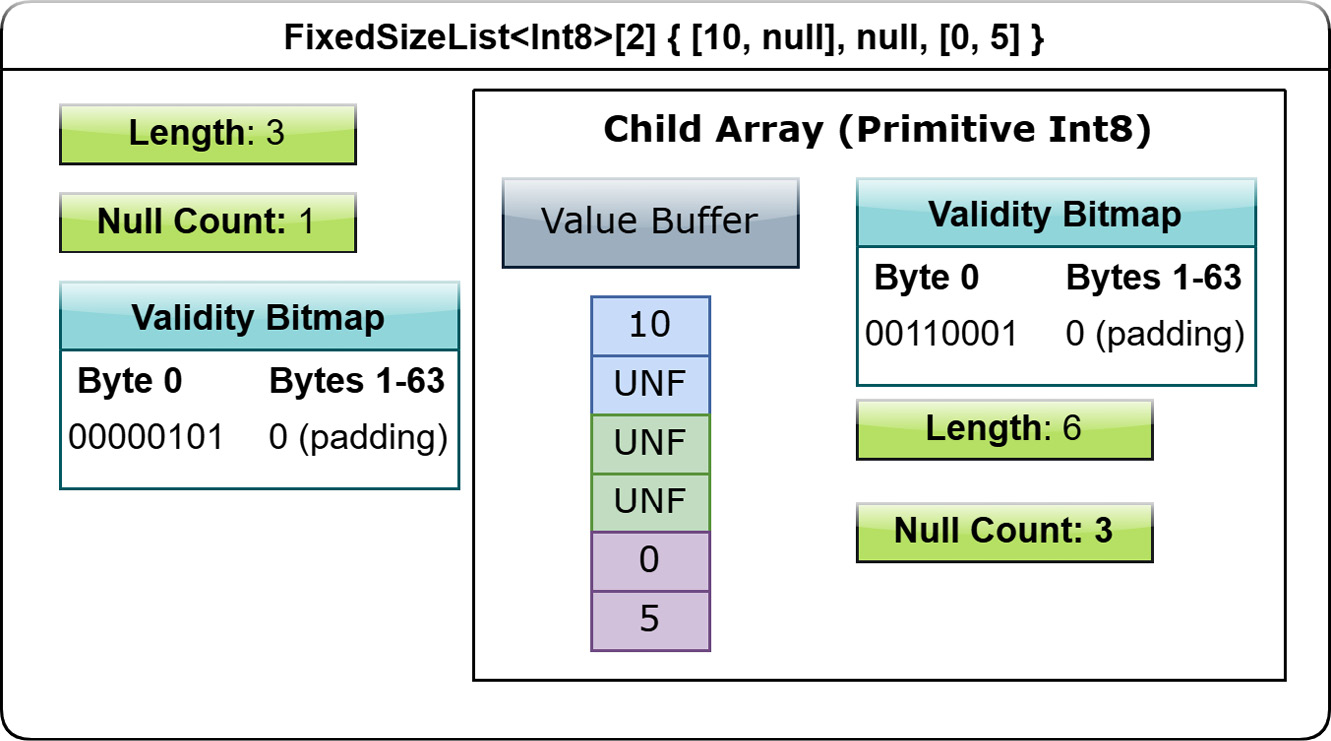
Figure 1.11 – Layout of fixed-size list array

What's the benefit of FixedSizeList versus List? Look back at the two diagrams again! Determining the values for a given slot of FixedSizeList doesn't require any lookups into a separate offsets buffer, making it more efficient if you know that your lists will always be a specific size. As a result, you also save space by not needing the extra memory for an offsets buffer at all!

Important Note

One thing to keep in mind is the semantic difference between a null value and an empty list. Using JSON notation, the difference is equivalent to the difference between null and []. The meaning of such a difference would be up to a particular application to decide, but it's important to note that a null list is not identical to an empty list, even though the only difference in the physical representation is the bit in the validity bitmap.

Phew! That was a lot. We're almost done!

Struct arrays

The next type on our tour of the Arrow format is the struct type's layout. A struct is a nested type that has an ordered sequence of fields that can all have their own distinct types. It's semantically very similar to a simple object with attributes that you might find in a variety of programming languages. Each field must have its own UTF-8 encoded name, and these field names are part of the metadata for defining a struct type. Instead of having any physical storage allocated for its values, a struct array has one child array for each of its fields. All of these children arrays are independent and don't need to be adjacent to each other in memory; remember our goal is column- (or field-) oriented, not row-oriented. A struct array must, however, have a validity bitmap if it contains one or more null struct values. It can still contain a validity bitmap if there are no null values, it's just optional in that case.

Let's use the example of a struct with the following structure: Struct<name: VarBinary, age: Int32>. An array of this type would have two child arrays, one VarBinary array (a variable-sized binary layout), and one 4-byte primitive value array having a logical type of Int32. With this definition, we can map out a representation of the array: [{"joe", 1}, {null, 2}, null, {"mark", 4}].

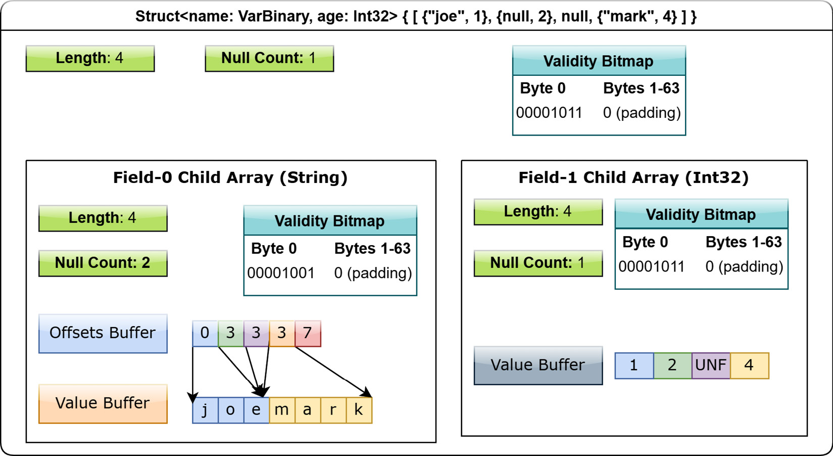
Figure 1.12 – Layout of struct array

When an entire slot of the struct array is set to null, the null is represented in the parent's validity bitmap, which is different from a particular value in a child array being null. In Figure 1.12, the child arrays each have a slot for the null struct in which they could have any value at all, but would be hidden by the struct array's validity bitmap marking the corresponding struct slot as null and taking priority over the children.

Union arrays – sparse and dense

For the case when a single column could have multiple types, there exists the Union type array. Whereas the struct array is an ordered sequence of fields, a union type is an ordered sequence of types. The value in each slot of the array could be of any of these types, which are named like struct fields and included in the metadata of the type. Unlike other layouts, the union type does not have its own validity bitmap. Instead, each slot's validity is determined by the children, which are composed to create the union array itself. There are two distinct union layouts that can be used when creating an array: dense and sparse, each optimized for a different use case.

A dense union represents a mixed-type array with 5 bytes of overhead for each value, and contains the following structures:

• One child array for each type
• A types buffer: A buffer of 8-bit signed integers, with each value representing the type ID for the corresponding slot, indicating which child vector to read from for that slot
• An offsets buffer: A buffer of signed 32-bit integers, indicating the offset into the corresponding child's array for the type in each slot

The dense union allows for the common use case of a union of structs with non-overlapping fields: Union<s1: Struct1, s2: Struct2, s3: Struct3……>. Here's an example of the layout for a union of type Union<f: float, i: int32> with the values [{f=1.2}, null, {f=3.4}, {i=5}]:

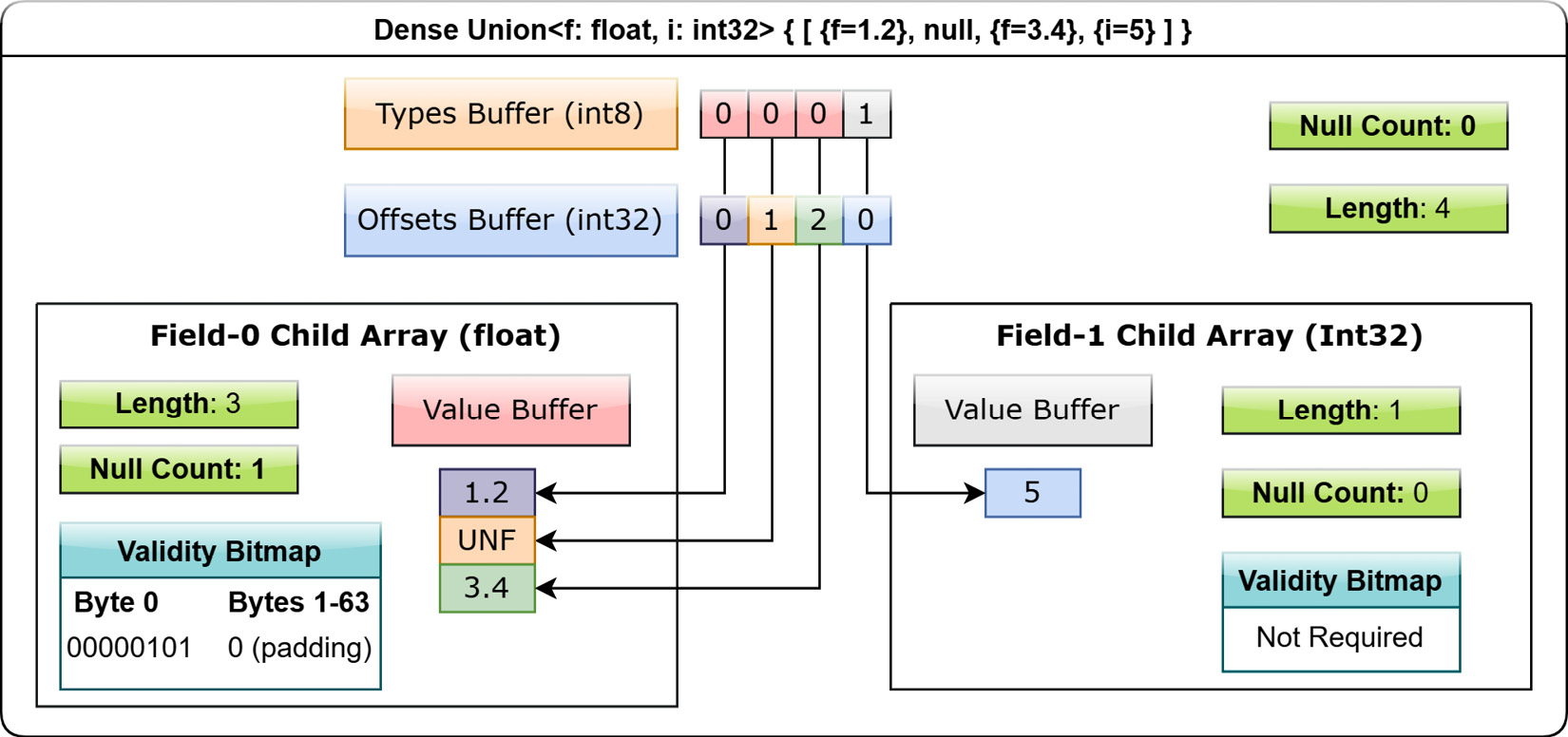
Figure 1.13 – Layout of dense union array

A sparse union has the same structure as the dense, except without an offsets array, as each child array is equal in length to the union itself. Figure 1.14 shows the same union array from Figure 1.13 as a sparse union array. There's no offsets buffer; both children are the same length of 4 as opposed to being different lengths:

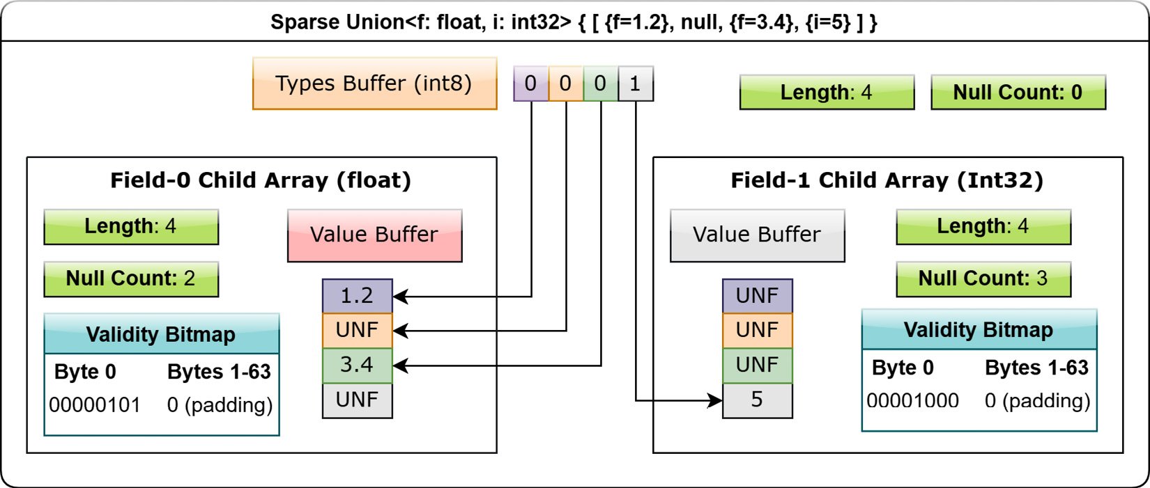
Figure 1.14 – Layout of sparse union array

Even though a sparse union takes up significantly more space compared to a dense union, it has some advantages for specific use cases. In particular, a sparse union is much more easily used with vectorized expression evaluation in many cases, and a group of equal length arrays can be interpreted as a union by only having to define the types buffer. When interpreting a sparse union, only the slot in a child indicated by the types array is considered; the rest of the unselected values are ignored and could be anything.

Dictionary-encoded arrays

Next, we arrive at the layout for dictionary-encoded arrays. If you have data that has many repeated values, then significant space can potentially be saved by using dictionary encoding to represent the data values as integers referencing indexes into a dictionary that usually consists of unique values. Since a dictionary is an optional property on any array, any array can be dictionary-encoded. The layout of a dictionary-encoded array is that of a primitive integer array of non-negative integers, which each represent the index in the dictionary. The dictionary itself is a separate array with its own respective layout of the appropriate type.

For example, let's say you have the following array: ["foo", "bar", "foo", "bar", null, "baz"]. Without dictionary encoding, we'd have an array that looks like this:

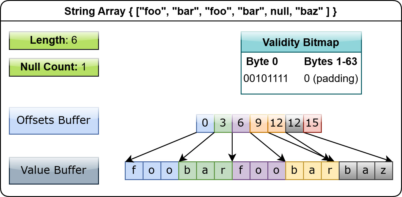
Figure 1.15 – String array without dictionary encoding

If we add dictionary encoding, we just need to get the unique values and create an array of indexes that references a dictionary array. The common case is to use int32, but any integral type would work:

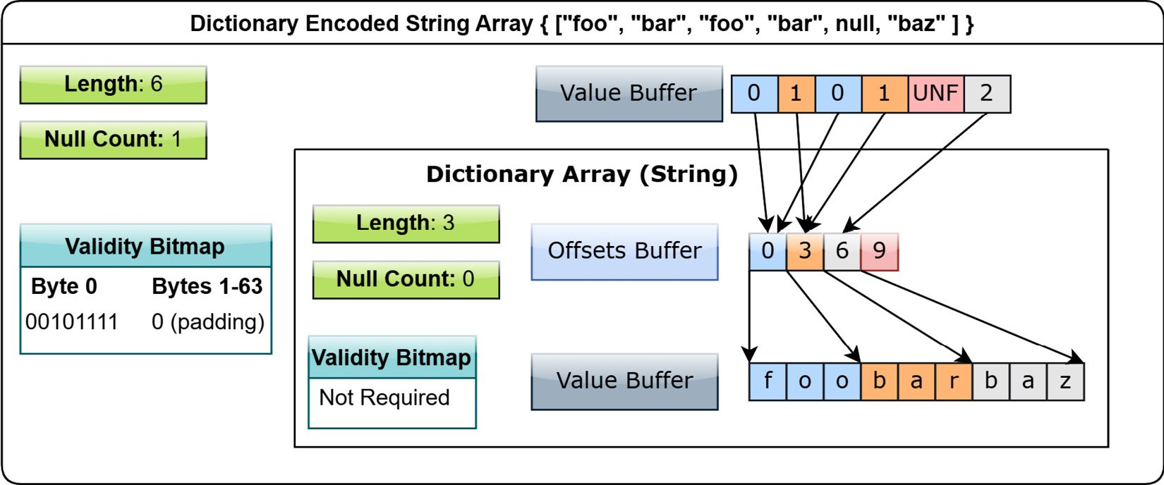
Figure 1.16 – Dictionary-encoded string array

For this trivial example, it's not particularly enticing, but it's very clear how, in the case of an array with a lot of repeated values, this could be a significant memory usage improvement. You can even perform operations directly on a dictionary array, updating the dictionary if needed or even swapping out the dictionary and replacing it.

As written in the specification, a dictionary is allowed to contain duplicates and even null values. However, the null count of a dictionary-encoded array is dictated by the validity bitmap of the indices, regardless of any nulls that might be in the dictionary itself.

Null arrays

Finally, there is only one more layout, but it's simple: a null array. A null array is an optimized layout for an array of all null values, with the type set to null; the only thing it contains is a length, no validity bitmap, and no data buffer.

How to speak Arrow

We've mentioned a few of the logical types already when describing the physical layouts, but let's get a full description of the current available logical types, as of Arrow release version 7.0.0, for your reading pleasure. In general, the logical types are what is referred to as the data type of an array in the libraries rather than the physical layouts. These types are what you will generally see when working with Arrow arrays in code:

• Null logical type: Null physical type
• Boolean: Primitive array with data represented as a bitmap
• Primitive integer types: Primitive, fixed-size array layout:
  • Int8, Uint8, Int16, Uint16, Int32, Uint32, Int64, and Uint64
• Floating-point types: Primitive fixed-size array layout:
  • Float16, Float32 (float), and Float64 (double)
• VarBinary types: Variable length binary physical layout:
  • Binary and String (UTF-8)
  • LargeBinary and LargeString (variable length binary with 64-bit offsets)
• Decimal128 and Decimal256: 128-bit and 256-bit fixed-size primitive arrays with metadata to specify the precision and scale of the values
• Fixed-size binary: Fixed-size binary physical layout
• Temporal types: Primitive fixed-size array physical layout
  • Date types: Dates with no time information:
    • Date32: 32-bit integers representing the number of days since the Unix epoch (1970-01-01)
    • Date64: 64-bit integers representing milliseconds since the Unix epoch (1970-01-01)
  • Time types: Time information with no date attached:
    • Time32: 32-bit integers representing elapsed time since midnight as seconds or milliseconds. A unit specified by metadata.
    • Time64: 64-bit integers representing elapsed time since midnight as microseconds or nanoseconds. A unit specified by metadata.
  • Timestamp: 64-bit integer representing the time since the Unix epoch, not including leap seconds. Metadata defines the unit (seconds, milliseconds, microseconds, or nanoseconds) and, optionally, a time zone as a string.
  • Interval types: An absolute length of time in terms of calendar artifacts:
    • YearMonth: Number of elapsed whole months as a 32-bit signed integer.
    • DayTime: Number of elapsed days and milliseconds as two consecutive 4-byte signed integers (8-bytes total per value).
    • MonthDayNano: Elapsed months, days, and nanoseconds stored as contiguous 16-byte blocks. Months and days as two 32-bit integers and nanoseconds since midnight as a 64-bit integer.
    • Duration: An absolute length of time not related to calendars as a 64-bit integer and a unit specified by metadata indicating seconds, milliseconds, microseconds, or nanoseconds.
• List and FixedSizeList: Their respective physical layouts:
  • LargeList: A list type with 64-bit offsets
• Struct, DenseUnion, and SparseUnion types: Their respective physical layouts
• Map: A logical type that is physically represented as List<entries: Struct<key: K, value: V>>, where K and V are the respective types of the keys and values in the map:
  • Metadata is included indicating whether or not the keys are sorted.

Whenever speaking about the types of an array from an application or semantic standpoint, we will always be using the types indicated in the preceding list to describe them. As you can see, the logical types make it very easy to represent both flat and hierarchical types of data. Now that we've covered the physical memory layouts, let's have a quick word about the versioning and stability of the Arrow format and libraries.