Reader small image

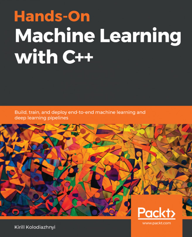
You're reading from  Hands-On Machine Learning with C++

Product typeBook
Published inMay 2020
Reading LevelIntermediate
PublisherPackt
ISBN-139781789955330
Edition1st Edition
Languages
Tools
Right arrow
Author (1)
Kirill Kolodiazhnyi
Kirill Kolodiazhnyi
author image
Kirill Kolodiazhnyi

Kirill Kolodiazhnyi is a seasoned software engineer with expertise in custom software development. He has several years of experience building machine learning models and data products using C++. He holds a bachelor degree in Computer Science from the Kharkiv National University of Radio-Electronics. He currently works in Kharkiv, Ukraine where he lives with his wife and daughter.
Read more about Kirill Kolodiazhnyi

Right arrow

An overview of linear algebra

The concepts of linear algebra are essential for understanding the theory behind ML because they help us understand how ML algorithms work under the hood. Also, most ML algorithm definitions use linear algebra terms.

Linear algebra is not only a handy mathematical instrument, but also the concepts of linear algebra can be very efficiently implemented with modern computer architectures. The rise of ML, and especially deep learning, began after significant performance improvement of the modern Graphics Processing Unit (GPU). GPUs were initially designed to work with linear algebra concepts and massive parallel computations used in computer games. After that, special libraries were created to work with general linear algebra concepts. Examples of libraries that implement basic linear algebra routines are Cuda and OpenCL, and one example of a specialized linear algebra library is cuBLAS. Moreover, it became more common to use general-purpose graphics processing units (GPGPUs) because these turn the computational power of a modern GPU into a powerful general-purpose computing resource.

Also, Central Processing Units (CPUs) have instruction sets specially designed for simultaneous numerical computations. Such computations are called vectorized, and common vectorized instruction sets are AVx, SSE, and MMx. There is also a term Single Instruction Multiple Data (SIMD) for these instruction sets. Many numeric linear algebra libraries, such as Eigen, xtensor, VienaCL, and others, use them to improve computational performance.

Learning the concepts of linear algebra

Linear algebra is a big area. It is the section of algebra that studies objects of a linear nature: vector (or linear) spaces, linear representations, and systems of linear equations. The main tools used in linear algebra are determinants, matrices, conjugation, and tensor calculus.

To understand ML algorithms, we only need a small set of linear algebra concepts. However, to do researches on new ML algorithms, a practitioner should have a deep understanding of linear algebra and calculus.

The following list contains the most valuable linear algebra concepts for understanding ML algorithms:

  • Scalar: This is a single number.
  • Vector: This is an array of ordered numbers. Each element has a distinct index. Notation for vectors is a bold lowercase typeface for names and an italic typeface with a subscript for elements, as shown in the following example:
  • Matrix: This is a two-dimensional array of numbers. Each element has a distinct pair of indices. Notation for matrices is a bold uppercase typeface for names and an italic but not bold typeface with a comma-separated list of indices in subscript for elements, as shown in the following example:
  • Tensor: This is an array of numbers arranged in a multidimensional regular grid, and represents generalizations of matrices. It is like a multidimensional matrix. For example, tensor A with dimensions 2 x 2 x 2 can look like this:

Linear algebra libraries and ML frameworks usually use the concept of a tensor instead of a matrix because they implement general algorithms, and a matrix is just a special case of a tensor with two dimensions. Also, we can consider a vector as a matrix of size n x 1.

Basic linear algebra operations

The most common operations used for programming linear algebra algorithms are the following ones:

  • Element-wise operations: These are performed in an element-wise manner on vectors, matrices, or tensors of the same size. The resulting elements will be the result of operations on corresponding input elements, as shown here:

The following example shows the element-wise summation:

  • Dot product: There are two types of multiplications for tensor and matrices in linear algebra—one is just element-wise, and the second is the dot product. The dot product deals with two equal-length series of numbers and returns a single number. This operation applied on matrices or tensors requires that the matrix or tensor A has the same number of columns as the number of rows in the matrix or tensor B. The following example shows the dot-product operation in the case when A is an n x m matrix and B is an m x p matrix:

  • Transposing: The transposing of a matrix is an operation that flips the matrix over its diagonal, which leads to the flipping of the column and row indices of the matrix, resulting in the creation of a new matrix. In general, it is swapping matrix rows with columns. The following example shows how transposing works:
  • Norm: This operation calculates the size of the vector; the result of this is a non-negative real number. The norm formula is as follows:

The generic name of this type of norm is norm for . Usually, we use more concrete norms such as an norm with p = 2, which is known as the Euclidean norm, and we can interpret it as the Euclidean distance between points. Another widely used norm is the squared norm, whose calculation formula is . The squared norm is more suitable for mathematical and computational operations than the norm. Each partial derivative of the squared norm depends only on the corresponding element of x, in comparison to the partial derivatives of the norm which depends on the entire vector; this property plays a vital role in optimization algorithms. Another widely used norm operation is the norm with p=1, which is commonly used in ML when we care about the difference between zero and nonzero elements.

  • Inverting: The inverse matrix is such a matrix that , where I is an identity matrix. The identity matrix is a matrix that does not change any vector when we multiply that vector by that matrix.

We considered the main linear algebra concepts as well as operations on them. Using this math apparatus, we can define and program many ML algorithms. For example, we can use tensors and matrices to define training datasets for training, and scalars can be used as different types of coefficients. We can use element-wise operations to perform arithmetic operations with a whole dataset (a matrix or a tensor). For example, we can use element-wise multiplication to scale a dataset. We usually use transposing to change a view of a vector or matrix to make them suitable for the dot-product operation. The dot product is usually used to apply a linear function with weights expressed as matrix coefficients to a vector; for example, this vector can be a training sample. Also, dot-product operations are used to update model parameters expressed as matrix or tensor coefficients according to an algorithm.

The norm operation is often used in formulas for loss functions because it naturally expresses the distance concept and can measure the difference between target and predicted values. The inverse matrix is a crucial concept for the analytical solving of linear equations systems. Such systems often appear in different optimization problems. However, calculating the inverse matrix is very computationally expensive.

Tensor representation in computing

We can represent tensor objects in computer memory in different ways. The most obvious method is a simple linear array in computer memory (random-access memory, or RAM). However, the linear array is also the most computationally effective data structure for modern CPUs. There are two standard practices to organize tensors with a linear array in memory: row-major ordering and column-major ordering. In row-major ordering, we place consecutive elements of a row in linear order one after the other, and each row is also placed after the end of the previous one. In column-major ordering, we do the same but with the column elements. Data layouts have a significant impact on computational performance because the speed of traversing an array relies on modern CPU architectures that work with sequential data more efficiently than with non-sequential data. CPU caching effects are the reasons for such behavior. Also, a contiguous data layout makes it possible to use SIMD vectorized instructions that work with sequential data more efficiently, and we can use them as a type of parallel processing.

Different libraries, even in the same programming language, can use different ordering. For example, Eigen uses column-major ordering, but PyTorch uses row-major ordering. So, developers should be aware of internal tensor representation in libraries they use, and also take care of this when performing data loading or implementing algorithms from scratch.

Consider the following matrix:

Then, in the row-major data layout, members of the matrix will have the following layout in memory:

0

1

2

3

4

5

a11

a12

a13

a21

a22

a23

In the case of the column-major data layout, order layout will be the next, as shown here:

0

1

2

3

4

5

a11

a21

a12

a22

a13

a23

Linear algebra API samples

Consider some C++ linear algebra APIs (short for Application Program Interface), and look at how we can use them for creating linear algebra primitives and perform algebra operations with them.

Using Eigen

Eigen is a general-purpose linear algebra C++ library. In Eigen, all matrices and vectors are objects of the Matrix template class, and the vector is a specialization of the matrix type, with either one row or one column. Tensor objects are not presented in official APIs but exist as submodules.

We can define the type for a matrix with known dimensions and floating-point data type like this:

typedef Eigen::Matrix<float, 3, 3> MyMatrix33f;

We can define a vector in the following way:

typedef Eigen::Matrix<float, 3, 1> MyVector3f;

Eigen already has a lot of predefined types for vector and matrix objects—for example, Eigen::Matrix3f (floating-point 3x3 matrix type) or Eigen::RowVector2f (floating-point 1 x 2 vector type). Also, Eigen is not limited to matrices whose dimensions we know at compile time. We can define matrix types that will take the number of rows or columns at initialization during runtime. To define such types, we can use a special type variable for the Matrix class template argument named Eigen::Dynamic. For example, to define a matrix of doubles with dynamic dimensions, we can use the following definition:

typedef Eigen::Matrix<double, Eigen::Dynamic, Eigen::Dynamic> MyMatrix;

Objects initialized from the types we defined will look like this:

MyMatrix33f a;
MyVector3f v;
MyMatrix m(10,15);

To put some values into these objects, we can use several approaches. We can use special predefined initialization functions, as follows:

a = MyMatrix33f::Zero(); // fill matrix elements with zeros
a = MyMatrix33f::Identity(); // fill matrix as Identity matrix
v = MyVector3f::Random(); // fill matrix elements with random values

We can use the comma-initializer syntax, as follows:

a << 1,2,3,
4,5,6,
7,8,9;

This code construction initializes the matrix values in the following way:

We can use direct element access to set or change matrix coefficients. The following code sample shows how to use the () operator for such an operation:

a(0,0) = 3;

We can use the object of the Map type to wrap an existent C++ array or vector in the Matrix type object. This kind of mapping object will use memory and values from the underlying object, and will not allocate the additional memory and copy the values. The following snippet shows how to use the Map type:

int data[] = {1,2,3,4};
Eigen::Map<Eigen::RowVectorxi> v(data,4);
std::vector<float> data = {1,2,3,4,5,6,7,8,9};
Eigen::Map<MyMatrix33f> a(data.data());

We can use initialized matrix objects in mathematical operations. Matrix and vector arithmetic operations in the Eigen library are offered either through overloads of standard C++ arithmetic operators such as +, -, *, or through methods such as dot() and cross(). The following code sample shows how to express general math operations in Eigen:

using namespace Eigen;   
auto a = Matrix2d::Random();
auto b = Matrix2d::Random();
auto result = a + b;
result = a.array() * b.array(); // element wise multiplication
result = a.array() / b.array();
a += b;
result = a * b; // matrix multiplication
//Also it’s possible to use scalars:
a = b.array() * 4;

Notice that in Eigen, arithmetic operators such as operator+ do not perform any computation by themselves. These operators return an expression object, which describes what computation to perform. The actual computation happens later when the whole expression is evaluated, typically in the operator= arithmetic operator. It can lead to some strange behaviors, primarily if a developer uses the auto keyword too frequently.

Sometimes, we need to perform operations only on a part of the matrix. For this purpose, Eigen provides the block method, which takes four parameters: i,j,p,q. These parameters are the block size p,q and the starting point i,j. The following code shows how to use this method:

Eigen::Matrixxf m(4,4);
Eigen::Matrix2f b = m.block(1,1,2,2); // copying the middle part of matrix
m.block(1,1,2,2) *= 4; // change values in original matrix

There are two more methods to access rows and columns by index, which are also a type of block operation. The following snippet shows how to use the col and the row methods:

m.row(1).array() += 3;
m.col(2).array() /= 4;

Another important feature of linear algebra libraries is broadcasting, and Eigen supports this with the colwise and rowwise methods. Broadcasting can be interpreted as a matrix by replicating it in one direction. Take a look at the following example of how to add a vector to each column of the matrix:

Eigen::Matrixxf mat(2,4);
Eigen::Vectorxf v(2); // column vector
mat.colwise() += v;

This operation has the following result: .

Using xtensor

The xtensor library is a C++ library for numerical analysis with multidimensional array expressions. Containers of xtensor are inspired by NumPy, the Python array programming library. ML algorithms are mainly described using Python and NumPy, so this library can make it easier to move them to C++. The following container classes implement multidimensional arrays in the xtensor library.

The xarray type is a dynamically sized multidimensional array, as shown in the following code snippet:

std::vector<size_t> shape = { 3, 2, 4 };
xt::xarray<double, xt::layout_type::row_major> a(shape);

The xtensor type is a multidimensional array whose dimensions are fixed at compilation time. Exact dimension values can be configured in the initialization step, as shown in the following code snippet:

std::array<size_t, 3> shape = { 3, 2, 4 };
xt::xtensor<double, 3> a(shape);

The xtensor_fixed type is a multidimensional array with a dimension shape fixed at compile time, as shown in the following code snippet:

xt::xtensor_fixed<double, xt::xshape<3, 2, 4>> a;

The xtensor library also implements arithmetic operators with expression template techniques such as Eigen (this is a common approach for math libraries implemented in C++). So, the computation happens lazily, and the actual result is calculated when the whole expression is evaluated. The container definitions are also expressions. There is also a function to force an expression evaluation named xt::eval in the xtensor library.

There are different kinds of container initialization in the xtensor library.
Initialization of xtensor arrays can be done with C++ initializer lists, as follows:

        xt::xarray<double> arr1{{1.0, 2.0, 3.0},
{2.0, 5.0, 7.0},
{2.0, 5.0, 7.0}}; // initialize a 3x3 array

The xtensor library also has builder functions for special tensor types. The following snippet shows some of them:

std::vector<uint64_t> shape = {2, 2};
xt::ones(shape);
xt::zero(shape);
xt::eye(shape); //matrix with ones on the diagonal

Also, we can map existing C++ arrays into the xtensor container with the xt::adapt function. This function returns the object that uses the memory and values from the underlying object, as shown in the following code snippet:

std::vector<float> data{1,2,3,4};
std::vector<size_t> shape{2,2};
auto data_x = xt::adapt(data, shape);

We can use direct access to container elements, with the () operator, to set or change tensor values, as shown in the following code snippet:

std::vector<size_t> shape = {3, 2, 4};
xt::xarray<float> a = xt::ones<float>(shape);
a(2,1,3) = 3.14f;

The xtensor library implements linear algebra arithmetic operations through overloads of standard C++ arithmetic operators such as +, - and *. To use other operations such as dot-product operations, we have to link an application with the library named xtensor-blas. These operators are declared in the xt::linalg namespace.

The following code shows the use of arithmetic operations with the xtensor library:

auto a = xt::random::rand<double>({2,2});
auto b = xt::random::rand<double>({2,2});
auto c = a + b;
a -= b;
c = xt::linalg::dot(a,b);
c = a + 5;

To get partial access to the xtensor containers, we can use the xt::view function. The following sample shows how this function works:

xt::xarray<int> a{{1,  2,  3,  4},
{5, 6, 7, 8}
{9, 10, 11, 12}
{13, 14, 15, 16}};
auto b = xt::view(a, xt::range(1, 3), xt::range(1, 3));

This operation takes a rectangular block from the tensor, which looks like this:

The xtensor library implements automatic broadcasting in most cases. When the operation involves two arrays of different dimensions, it transmits the array with the smaller dimension across the leading dimension of the other array, so we can directly add a vector to a matrix. The following code sample shows how easy it is:

auto m = xt::random::rand<double>({2,2});
auto v = xt::random::rand<double>({2,1});
auto c = m + v;

Using Shark-ML

Shark-ML is a C++ ML library with rich functionality. It also provides an API for linear algebra routines.

There are four container classes for representing matrices and vectors in the Shark-ML library. Notice that the linear algebra functionality is declared in the remora namespace instead of the shark namespace, which is used for other routines.

The following code sample shows container classes that exist in the Shark-ML library, wherein the vector type is a dynamically sized array:

remora::vector<double> b(100, 1.0); // vector of size 100 and filled with 1.0

The compressed_vector type is a sparse array storing values in a compressed format.

The matrix type is a dynamically sized dense matrix, as shown in the following code snippet:

remora::matrix<double> C(2, 2); // 2x2 matrix

The compressed_matrix type is a sparse matrix storing values in a compressed format.

There are two main types of container initialization in the Shark-ML library.

We can initialize a container object with the constructor that takes the initializer list. The following code sample shows this:

remora::matrix<float> m_ones{{1, 1}, {1, 1}}; // 2x2 matrix

The second option is to wrap the existing C++ array into the container object and reuse its memory and values. The following code sample shows how to use the same array for the initialization of matrix and vector objects:

float data[]= {1,2,3,4};
remora::matrix<float> m(data, 2, 2);
remora::vector<float> v(data, 4);

Also, we can initialize values with direct access to the container elements, with the () operator. The following code sample shows how to set a value for matrix and vector objects:

remora::matrix<float> m(data, 2, 2);
m(0,0) = 3.14f;
remora::vector<float> v(data, 4);
v(0) = 3.14f;

The Shark-ML library implements linear algebra arithmetic operations through overloads of standard C++ arithmetic operators such as +, - and *. Some other operations such as the dot product are implemented as standalone functions.

The following code sample shows how to use arithmetic operations in the Shark-ML library:

remora::matrix<float> a(data, 2, 2);
remora::matrix<float> b(data, 2, 2);
auto c = a + b;
a -= b;
c = remora::prod(a,b);
c = a%b; // also dot product operation
c = a + 5;

We can use the following functions for partial access to the Shark ML containers:

  • subrange (x,i,j): This function returns a sub-vector of x with the elements xi,…, xj−1.
  • subrange (A,i,j,k,l): This function returns a sub-matrix of A with elements indicated by i,…, j−1 and k, …, l−1.
  • row (A,k): This function returns the kth row of A as a vector proxy.
  • column (A,k): This function returns the kth column of A as a vector proxy.
  • rows (A,k,l): This function returns the rows k,…,l−1 of A as a matrix proxy.
  • columns (A,k,l): This function returns the columns k,…, l−1 of A as a matrix proxy.

There is no broadcasting implementation in the Shark-ML library. Limited support of broadcasting exists only in the form of reduction functions (the set of functions that calculate one numeric value for a whole matrix or vector). There are two functions—the as_rows() and as_columns() function—that allow reduction operations to be performed independently on matrix rows or columns respectively. We can pass the result of these functions to any of the reduction functions. The following code sample shows how to perform summation reduction:

remora::matrix<float> m{{1, 2, 3, 4}, {5, 6, 7, 8}};
auto cols = remora::as_columns(m);
remora::sum(cols)

A different way to work with columns and rows independently is the use of partial access functions. The following code sample shows how to add the same vector to each of the matrix columns:

remora::vector<float> v{10, 10};
// Update matrix rows
for (size_t i = 0; i < m.size2(); ++i) {
remora::column(m, i) += v;
}

Using Dlib

Dlib is a modern C++ toolkit containing ML algorithms and tools for creating computer vision software in C++. Most of the linear algebra tools in Dlib deal with dense matrices. However, there is also limited support for working with sparse matrices and vectors. In particular, the Dlib tools represent sparse vectors using the containers from the C++ standard template library (STL).

There are two main container types in Dlib to work with linear algebra: the matrix and the vector classes. Matrix operations in Dlib are implemented using the expression templates technique, which allows them to eliminate the temporary matrix objects that would usually be returned from expressions such as M = A+B+C+D.

We can create a matrix sized at compile time in the following way, by specifying dimensions as template arguments:

Dlib::matrix<double,3,1> y;

Alternatively, we can create dynamically sized matrix objects. In such a case, we pass the matrix dimensions to the constructor, as shown in the following code snippet:

Dlib::matrix<double> m(3,3);

Later, we can change the size of this matrix, with the following method:

m.set_size(6,6);

We can initialize matrix values with a comma operator, as shown in the following code snippet:

m = 54.2,  7.4, 12.1,
1, 2, 3,
5.9, 0.05, 1;

As in the previous libraries, we can wrap an existing C++ array to the matrix object, as shown in the following code snippet:

double data[] = {1,2,3,4,5,6};
auto a = Dlib::mat(data, 2,3); // create matrix with size 2x3

Also, we can access matrix elements with the () operator to modify or get a particular value, as shown in the following code snippet:

m(1,2) = 3;

The Dlib library has a set of predefined functions to initialize a matrix with values such as identity matrix, 1s, or random values, as illustrated in the following code snippet:

auto a = Dlib::identity_matrix<double>(3);
auto b = Dlib::ones_matrix<double>(3,4);
auto c = Dlib::randm(3,4); // matrix with random values with size 3x3

Most linear algebra arithmetic operations in the Dlib library are implemented through overloads of standard C++ arithmetic operators such as +, -, *. Other complex operations are provided by the library as standalone functions.

The following example shows the use of arithmetic operations in the Dlib library:

auto c = a + b;
auto e = a * b; // real matrix multiplication
auto d = Dlib::pointwise_multiply(a, b); // element wise multiplication
a += 5;
auto t = Dlib::trans(a); // transpose matrix

To work with partial access to matrices, Dlib provides a set of special functions. The following code sample shows how to use some of them:

a = Dlib::rowm(b,0); // takes first row of matrix
a = Dlib::rowm(b,Dlib::range(0,1));//takes first two rows
a = Dlib::colm(b,0); // takes first column
a = Dlib::subm(b, range(1,2), range(1,2)); // takes a rectangular part from center
Dlib::set_subm(b,range(0,1), range(0,1)) = 7; // initialize part of the matrix
Dlib::set_subm(b,range(0,1), range(0,1)) += 7; // add a value to the part of the matrix

Broadcasting in the Dlib library can be modeled with set_rowm(), set_colm(), and set_subm() functions that give modifier objects for a particular matrix row, column, or a rectangular part of the original matrix. Objects returned from these functions support all set or arithmetic operations. The following code snippet shows how to add a vector to the columns:

Dlib::matrix<float, 2,1> x;
Dlib::matrix<float, 2,3> m;
Dlib::set_colm(b,Dlib::range(0,1)) += x;
Previous PageNext Page
You have been reading a chapter from
Hands-On Machine Learning with C++
Published in: May 2020Publisher: PacktISBN-13: 9781789955330
Register for a free Packt account to unlock a world of extra content!
A free Packt account unlocks extra newsletters, articles, discounted offers, and much more. Start advancing your knowledge today.
undefined
Unlock this book and the full library FREE for 7 days
Get unlimited access to 7000+ expert-authored eBooks and videos courses covering every tech area you can think of
Renews at $15.99/month. Cancel anytime

Author (1)

author image
Kirill Kolodiazhnyi

Kirill Kolodiazhnyi is a seasoned software engineer with expertise in custom software development. He has several years of experience building machine learning models and data products using C++. He holds a bachelor degree in Computer Science from the Kharkiv National University of Radio-Electronics. He currently works in Kharkiv, Ukraine where he lives with his wife and daughter.
Read more about Kirill Kolodiazhnyi