Statistical Modeling in Anaconda

In this chapter, we will first present the simplest statistical model: the one-factor linear model. To make the learning process more interesting, we will discuss an application of such a model: the famous financial model called the Capital Asset Pricing Model (CAPM). In terms of processing data, we will show you how to detect and remove missing values, and how to replace missing values with means or other values in R, Python, or Julia. Also, outliers would distort our statistical results. Thus, we need to know how to detect and deal with them. After that, we talk about multi-factor linear models. Again, to make our discussion more meaningful, we will discuss the famous Fama-French 3-factor and 5-factor linear models, and the Fama-French-Carhart 4-factor linear model. Then, we will discuss how to rank those different models, that is, how to measure...

Introduction to linear models

The one-factor linear model is the simplest way to show a relationship between two variables: y and x. In other words, we try to use x to explain y. The general form for a one-factor linear model is given here, where y_t is the dependent variable at time t, α is the intercept, β is the slope, x_t is the value of an independent variable at time t, and ε_t is a random term:

To run a linear regression, we intend to estimate the intercept (α) and the slope (β). One-factor means that the model has just one explanatory variable, that is, one independent variable of x, and linear means that when drawing a graph based on the equation (1), we would have a straight line. With the following R program, we could get a linear line:

> x<--10:10
> y<-2+1.5*x
> title<-"A straight line"
> plot(x,y,type='l...

Running a linear regression in R, Python, Julia, and Octave

The following code block shows how to run such a one-factor linear regression in R:

> set.seed(12345)
> x<-1:100
> a<-4
> beta<-5
> errorTerm<-rnorm(100)
> y<-a+beta*x+errorTerm
> lm(y~x)

The first line of set.seed(12345) guarantees that different users will get the same random numbers when the same seed() is applied, that is, 12345 in this case. The R function rnorm(n) is used to generate n random numbers from a standard normal distribution. Also, the two letters of the lm() function stand for linear model. The result is shown here:

Call: lm(formula = y ~ x)
Coefficients: 
(Intercept) x 
4.114 5.003

The estimated intercept is 4.11, while the estimated slope is 5.00. To get more information about the function, we can use the summary() function, shown in the following code:

> summary(lm(y...

Critical value and the decision rule

A T-test is any statistical hypothesis test in which the test statistic follows a student's T-distribution under the null hypothesis. It can be used to determine whether two sets of data are significantly different from each other. For a one-sample T-test and for the null hypothesis that the mean is equal to a specified value μ₀, we use the following statistic, where t is the T-value, is the sample mean, μ₀ is the our assumed return mean, σ is the sample standard deviation of the sample, n is the sample size, and S.E. is the standard error:

The degrees of freedom used in this test are n - 1. The critical T-value is used to accept or reject the null hypothesis. The decision rule is given here:

In the previous section, we mentioned two critical values: 2 for a T-value and 0.05 for a P-value....

F-test, critical value, and the decision rule

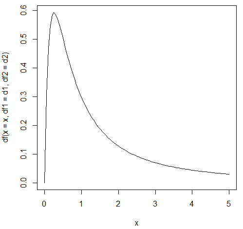
In the previous examples, we saw the F-value for the performance of the whole model. Now, let's look at the F-distribution. Assume that x₁ and x₂ are two independent random variables with the Chi-Square distribution with df₁ and df₂ degrees of freedom, respectively. The ratio of x₁/df₁ divided by x₂/df₂ would follow an F-distribution:

An R program to draw a graph for the F distribution with (10, 2) degrees of freedom is shown here:

> d1<-4 
> d2<-2 
> n<-100 
> x = seq(0, 5, length = n) 
> plot(x, df(x = x, df1 = d1, df2 = d2),type='l') 

The related plot is shown here:

The following R program shows the critical value for a given α of 0.1 and (1, 2) degrees of freedom:

> alpha<-0.1
> d1<-1
> d2<-1
> qf(1-alpha,df1=d1,df2=d2)
[1] 39.86346

The following Python program...

Dealing with missing data

There are many ways to deal with missing records. The simplest one is to delete them. This is especially true when we have a relative large dataset. One potential issue is that our final dataset should not be changed in any fundamental way after we delete the missing data. In other words, if the missing records happened in a random way, then simply deleting them would not generate a biased result.

Removing missing data

The following R program uses the na.omit() function:

> x<-c(NA,1,2,50,NA) 
> y<-na.omit(x) 
> mean(x) 
[1] NA 
> mean(y) 
[1] 17.66667 

Another R function called na.exclude() could be used as well. The following Python program removes all sp.na code:

import scipy as...

Detecting outliers and treatments

First, a word of caution: one person's waste might be another person's treasure, and this is true for outliers. For example, for the week of 2/5/2018 to 2/15/2018, the Dow Jones Industrial Average (DJIA) suffers a huge loss. Cheng and Hum (2018) show that the index travels more than 22,000 points, as shown in the following table:

Weekday	Points
Monday	5,113
Tuesday	5,460
Wednesday	2,886
Thursday	3,369
Friday	5,425
Total	22,253

Table 5.1 Dow Jones industrial average points traveled

If we want to study the relationship between a stock and the DJIA index, the observations might be treated as outliers. However, when studying the topic related to the impact of the market on individual stocks, we should pay special attention to those observations. In other words, those observations should not be...

Several multivariate linear models

As we mentioned at the beginning of the chapter, we could show several applications of multivariable linear models. The first one is a three-factor linear model. The general formula is quite similar to the one-factor linear model, shown here:

The definitions are the same as before. The only difference is that we have three independent variables instead of one. Our objective is to estimate four parameters, one intercept plus three coefficients:

For example, the equation of the famous Fama-French 3-factor model is given, where R_i is the stock i's return and R_m is the market return. SMB (Small Minus Big) is defined as the returns of the small portfolios minus the returns of the big portfolios and HML (High Minus Low) is the difference of returns of high book-to-market portfolios minus the returns of low book-to-market portfolios. (See the...

Collinearity and its solution

In statistics, multicollinearity, or collinearity, is a phenomenon in which one independent variable (predictor variable) in a multiple regression model can be linearly predicted from the others with a substantial degree of accuracy. Collinearity tends to inflate the variance of at least one estimated regression coefficient. This could cause some regression coefficients to have the wrong sign. Those issues would make our regression results unreliable. Therefore, how can we detect the potential problem? One way is that we could simply look at the correlation between each pair of independent variables. If their correlation is close to ±1, then we might have such an issue:

>con<-url("http://canisius.edu/~yany/RData/ff3monthly.RData") 
>load(con) 
> head(.ff3monthly) 
        DATE  MKT_RF     SMB     HML     RF 
1 1926-07-01...

A model's performance measure

In this chapter, we looked at several applications of linear models, including CAPM, the Fama-French 3-factor linear model, the Fama-French-Carhart 4-factor linear model, and the Fama-French 5-factor linear model. Obviously, CAPM is the simplest one since it only involves a market index as the explanatory variable. One question remains though: which model is the best? In other words, how do we rank these models and how is their performance measured? When running linear regressions, the output will show both the R² and adjusted R². When comparing models with different numbers of independent variables, the adjusted R² is a better measure since it is adjusted by the number of input variables. However, note we should not depend only on the adjusted R² since this is in the sample measure. In other words, a higher adjusted R² simply means that based...

Summary

In this chapter, we have explained many important issues related to statistics, such as T-distribution, F-distribution, T-tests, F-tests, and other hypothesis tests. We have also discussed linear regression, how to deal with missing data, how to treat outliers, collinearity and its treatments, and how to run a multi-variable linear regression.

In Chapter 6, Managing Packages, we will discuss the importance of managing package; how to find out about all packages available for R, Python, and Julia; and how to find the manual for each package. In addition, we will discuss the issue of package dependency and how to make our programming a little easier when dealing with packages.

Review questions and exercises

1. What is the definition of a single-factor linear model?
2. How many independent variables are there in a single-factor model?
3. What does it mean for something to be statically different from zero?
4. What are the critical T-values and P-values to tell whether an estimate is statistically significant?
5. When the significant level is 1%, what is the critical T-value when there are 30 degrees of freedom?

6. What is the difference between a one-sided test and a two-sided test?
7. What are the corresponding missing codes for missing data items in R, Python, and Julia?
8. How do we treat missing variables if our sample is big? How about if our sample is small?
9. How do we generally detect outliners and deal with them?
10. How do we generate a correlated return series? For example, write an R program to generate 5-year monthly returns for two stocks with a fixed correlation...