Chapter 5. Time Series

Time series typically consist of a sequence of data points coming from measurements taken over time. This kind of data is very common and occurs in a multitude of fields.

A business executive is interested in stock prices, prices of goods and services or monthly sales figures. A meteorologist takes temperature measurements several times a day and also keeps records of precipitation, humidity, wind direction and force. A neurologist can use electroencephalography to measure electrical activity of the brain along the scalp. A sociologist can use campaign contribution data to learn about political parties and their supporters and use these insights as an argumentation aid. More examples for time series data can be enumerated almost endlessly.

Time series primer

In general, time series serve two purposes. First, they help us to learn about the underlying process that generated the data. On the other hand, we would like to be able to forecast future values of the same or related series using existing data. When we measure temperature, precipitation or wind, we would like to learn more about more complex things, such as weather or the climate of a region and how various factors interact. At the same time, we might be interested in weather forecasting.

In this chapter we will explore the time series capabilities of Pandas. Apart from its powerful core data structures – the series and the DataFrame – Pandas comes with helper functions for dealing with time related data. With its extensive built-in optimizations, Pandas is capable of handling large time series with millions of data points with ease.

We will gradually approach time series, starting with the basic building blocks of date and time objects.

Working with date and time objects

Python supports date and time handling in the date time and time modules from the standard library:

>>> import datetime
>>> datetime.datetime(2000, 1, 1)
datetime.datetime(2000, 1, 1, 0, 0)

Sometimes, dates are given or expected as strings, so a conversion from or to strings is necessary, which is realized by two functions: strptime and strftime, respectively:

>>> datetime.datetime.strptime("2000/1/1", "%Y/%m/%d")
datetime.datetime(2000, 1, 1, 0, 0)
>>> datetime.datetime(2000, 1, 1, 0, 0).strftime("%Y%m%d")
'20000101'

Real-world data usually comes in all kinds of shapes and it would be great if we did not need to remember the exact date format specifies for parsing. Thankfully, Pandas abstracts away a lot of the friction, when dealing with strings representing dates or time. One of these helper functions is to_datetime:

>>> import pandas as pd
>>> import numpy as np
>>> pd.to_datetime("4th of...

Resampling time series

Resampling describes the process of frequency conversion over time series data. It is a helpful technique in various circumstances as it fosters understanding by grouping together and aggregating data. It is possible to create a new time series from daily temperature data that shows the average temperature per week or month. On the other hand, real-world data may not be taken in uniform intervals and it is required to map observations into uniform intervals or to fill in missing values for certain points in time. These are two of the main use directions of resampling: binning and aggregation, and filling in missing data. Downsampling and upsampling occur in other fields as well, such as digital signal processing. There, the process of downsampling is often called decimation and performs a reduction of the sample rate. The inverse process is called interpolation, where the sample rate is increased. We will look at both directions from a data analysis angle.

Downsampling time series data

Downsampling reduces the number of samples in the data. During this reduction, we are able to apply aggregations over data points. Let's imagine a busy airport with thousands of people passing through every hour. The airport administration has installed a visitor counter in the main area, to get an impression of exactly how busy their airport is.

They are receiving data from the counter device every minute. Here are the hypothetical measurements for a day, beginning at 08:00, ending 600 minutes later at 18:00:

>>> rng = pd.date_range('4/29/2015 8:00', periods=600, freq='T')
>>> ts = pd.Series(np.random.randint(0, 100, len(rng)), index=rng)
>>> ts.head()
2015-04-29 08:00:00     9
2015-04-29 08:01:00    60
2015-04-29 08:02:00    65
2015-04-29 08:03:00    25
2015-04-29 08:04:00    19

To get a better picture of the day, we can downsample this time series to larger intervals, for example, 10 minutes. We can choose an aggregation function...

Upsampling time series data

In upsampling, the frequency of the time series is increased. As a result, we have more sample points than data points. One of the main questions is how to account for the entries in the series where we have no measurement.

Let's start with hourly data for a single day:

>>> rng = pd.date_range('4/29/2015 8:00', periods=10, freq='H')
>>> ts = pd.Series(np.random.randint(0, 100, len(rng)), index=rng)
>>> ts.head()
2015-04-29 08:00:00    30
2015-04-29 09:00:00    27
2015-04-29 10:00:00    54
2015-04-29 11:00:00     9
2015-04-29 12:00:00    48
Freq: H, dtype: int64

If we upsample to data points taken every 15 minutes, our time series will be extended with NaN values:

>>> ts.resample('15min')
>>> ts.head()
2015-04-29 08:00:00    30
2015-04-29 08:15:00   NaN
2015-04-29 08:30:00   NaN
2015-04-29 08:45:00   NaN
2015-04-29 09:00:00    27

There are various ways to deal with missing values, which can be controlled by the fill_method...

Time zone handling

While, by default, Pandas objects are time zone unaware, many real-world applications will make use of time zones. As with working with time in general, time zones are no trivial matter: do you know which countries have daylight saving time and do you know when the time zone is switched in those countries? Thankfully, Pandas builds on the time zone capabilities of two popular and proven utility libraries for time and date handling: pytz and dateutil:

>>> t = pd.Timestamp('2000-01-01')
>>> t.tz is None
True

To supply time zone information, you can use the tz keyword argument:

>>> t = pd.Timestamp('2000-01-01', tz='Europe/Berlin')
>>> t.tz
<DstTzInfo 'Europe/Berlin' CET+1:00:00 STD>

This works for ranges as well:

>>> rng = pd.date_range('1/1/2000 00:00', periods=10, freq='D', tz='Europe/London')
>>> rng
DatetimeIndex(['2000-01-01', '2000-01-02', '2000-01-03', '2000-01-04', '2000-01-05', '2000-01-06', '2000-01-07...

Timedeltas

Along with the powerful timestamp object, which acts as a building block for the DatetimeIndex, there is another useful data structure, which has been introduced in Pandas 0.15 – the Timedelta. The Timedelta can serve as a basis for indices as well, in this case a TimedeltaIndex.

Timedeltas are differences in times, expressed in difference units. The Timedelta class in Pandas is a subclass of datetime.timedelta from the Python standard library. As with other Pandas data structures, the Timedelta can be constructed from a variety of inputs:

>>> pd.Timedelta('1 days')
Timedelta('1 days 00:00:00')
>>> pd.Timedelta('-1 days 2 min 10s 3us')
Timedelta('-2 days +23:57:49.999997')
>>> pd.Timedelta(days=1,seconds=1)
Timedelta('1 days 00:00:01')

As you would expect, Timedeltas allow basic arithmetic:

>>> pd.Timedelta(days=1) + pd.Timedelta(seconds=1)
Timedelta('1 days 00:00:01')

Similar to to_datetime, there is a to_timedelta function that can parse strings...

Time series plotting

Pandas comes with great support for plotting, and this holds true for time series data as well.

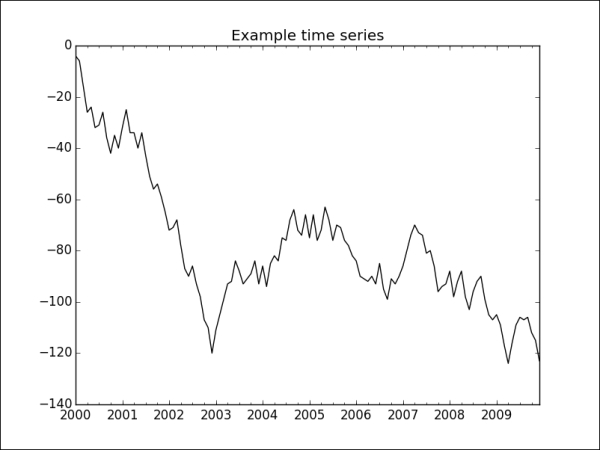
As a first example, let's take some monthly data and plot it:

>>> rng = pd.date_range(start='2000', periods=120, freq='MS')
>>> ts = pd.Series(np.random.randint(-10, 10, size=len(rng)), rng).cumsum()
>>> ts.head()
2000-01-01    -4
2000-02-01    -6
2000-03-01   -16
2000-04-01   -26
2000-05-01   -24
Freq: MS, dtype: int64

Since matplotlib is used under the hood, we can pass a familiar parameter to plot, such as c for color, or title for the chart title:

>>> ts.plot(c='k', title='Example time series')
>>> plt.show()

The following figure shows an example time series plot:

We can overlay an aggregate plot over 2 and 5 years:

>>> ts.resample('2A').plot(c='0.75', ls='--')
>>> ts.resample('5A').plot(c='0.25', ls='-.')

The following figure shows the resampled 2-year plot:

The following figure shows the resample 5-year plot...

Summary

In this chapter we showed how you can work with time series in Pandas. We introduced two index types, the DatetimeIndex and the TimedeltaIndex and explored their building blocks in depth. Pandas comes with versatile helper functions that take much of the pain out of parsing dates of various formats or generating fixed frequency sequences. Resampling data can help get a more condensed picture of the data, or it can help align various datasets of different frequencies to one another. One of the explicit goals of Pandas is to make it easy to work with missing data, which is also relevant in the context of upsampling.

Finally, we showed how time series can be visualized. Since matplotlib and Pandas are natural companions, we discovered that we can reuse our previous knowledge about matplotlib for time series data as well.

In the next chapter, we will explore ways to load and store data in text files and databases.

Prac tice examples

Exercise 1: Find one or two real-world examples for...