Reader small image

You're reading from  Generative Adversarial Networks Projects

Product typeBook
Published inJan 2019
Reading LevelIntermediate
PublisherPackt
ISBN-139781789136678
Edition1st Edition
Languages
Right arrow
Author (1)
Kailash Ahirwar
Kailash Ahirwar
author image
Kailash Ahirwar

Kailash Ahirwar is a machine learning and deep learning enthusiast. He has worked in many areas of Artificial Intelligence (AI), ranging from natural language processing and computer vision to generative modeling using GANs. He is a co-founder and CTO of Mate Labs. He uses GANs to build different models, such as turning paintings into photos and controlling deep image synthesis with texture patches. He is super optimistic about AGI and believes that AI is going to be the workhorse of human evolution.
Read more about Kailash Ahirwar

Right arrow

The detailed architecture of a GAN

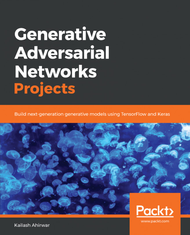
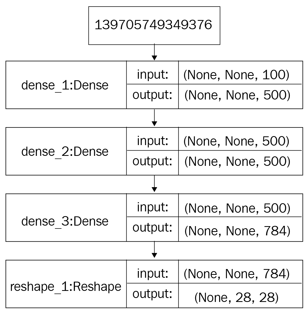
The architecture of a GAN has two basic elements: the generator network and the discriminator network. Each network can be any neural network, such as an Artificial Neural Network (ANN), a Convolutional Neural Network (CNN), a Recurrent Neural Network (RNN), or a Long Short Term Memory (LSTM). The discriminator has to have fully connected layers with a classifier at the end.

Let's take a closer look at the components of the architecture of a GAN. In this example, we will imagine that we are creating a dummy GAN.

The architecture of the generator

The generator network in our dummy GAN is a simple feed-forward neural network with five layers: an input layer, three hidden layers, and an output layer. Let's take a closer look at the configuration of the generator (dummy) network:

Layer #

Layer name

Configuration

1

Input layer

input_shape=(batch_size, 100), output_shape=(batch_size, 100)

2

Dense layer

neurons=500, input_shape=(batch_size, 100), output_shape=(batch_size, 500)

3

Dense layer

neurons=500, input_shape=(batch_size, 500), output_shape=(batch_size, 500)

4

Dense layer

neurons=784, input_shape=(batch_size, 500), output_shape=(batch_size, 784)

5

Reshape layer

input_shape=(batch_size, 784), output_shape=(batch_size, 28, 28)

The preceding table shows the configurations of the hidden layers, and also the input and output layers in the network.

The following diagram shows the flow of tensors and the input and output shapes of the tensors for each layer in the generator network:

The architecture of the generator network.

Let's discuss how this feed-forward neural network processes information during forward propagation of the data:

  • The input layer takes a 100-dimensional vector sampled from a Gaussian (normal) distribution and passes the tensor to the first hidden layer without any modifications.
  • The three hidden layers are dense layers with 500, 500, and 784 units, respectively. The first hidden layer (a dense layer) converts a tensor of a shape of (batch_size, 100) to a tensor of a shape of (batch_size, 500).
  • The second dense layer generates a tensor of a shape of (batch_size, 500).
  • The third hidden layer generates a tensor of a shape of (batch_size, 784).
  • In the last output layer, this tensor is reshaped from a shape of (batch_size, 784) to a shape of (batch_size, 28, 28). This means that our network will generate a batch of images, where one image will have a shape of (28, 28).

The architecture of the discriminator

The discriminator in our GAN is a feed-forward neural network with five layers, including an input and an output layer, and three dense layers. The discriminator network is a classifier and is slightly different from the generator network. It processes an image and outputs a probability of the image belonging to a particular class.

The following diagram shows the flow of tensors and the input and output shapes of the tensors for each layer in the discriminator network:

The architecture of the discriminator network

Let's discuss how the discriminator processes data in forward propagation during the training of the network:

  1. Initially, it receives an input of a shape of 28x28.
  2. The input layer takes the input tensor, which is a tensor with a shape of (batch_sizex28x28), and passes it to the first hidden layer without any modifications.
  3. Next, the flattening layer flattens the tensor to a 784-dimensional vector, which gets passed to the first hidden (dense) layer. The first and second hidden layers modify this to a 500-dimensional vector.
  4. The last layer is the output layer, which is again a dense layer, with one unit (a neuron) and sigmoid as the activation function. It outputs a single value, either a 0 or a 1. A value of 0 indicates that the provided image is fake, while a value of 1 indicates that the provided image is real.

Important concepts related to GANs

Now that we have understood the architecture of GANs, let's take a look at a brief overview of a few important concepts. We will first look at KL divergence. It is very important to understand JS divergence, which is an important measure to assess the quality of the models. We will then look at the Nash equilibrium, which is a state that we try to achieve during training. Finally, we will look closer at objective functions, which are very important to understand in order to implement GANs well.

Kullback-Leibler divergence

Kullback-Leibler divergence (KL divergence), also known as relative entropy, is a method used to identify the similarity between two probability distributions. It measures how one probability distribution p diverges from a second expected probability distribution q.

The equation used to calculate the KL divergence between two probability distributions p(x) and q(x) is as follows:

The KL divergence will be zero, or minimum, when p(x) is equal to q(x) at every other point.

Due to the asymmetric nature of KL divergence, we shouldn't use it to measure the distance between two probability distributions. It is therefore should not be used as a distance metric.

Jensen-Shannon divergence

The Jensen-Shannon divergence (also called the information radius (IRaD) or the total divergence to the average) is another measure of similarity between two probability distributions. It is based on KL divergence. Unlike KL divergence, however, JS divergence is symmetric in nature and can be used to measure the distance between two probability distributions. If we take the square root of the Jensen-Shannon divergence, we get the Jensen-Shannon distance, so it is therefore a distance metric.

The following equation represents the Jensen-Shannon divergence between two probability distributions, p and q:

In the preceding equation, (p+q) is the midpoint measure, while 
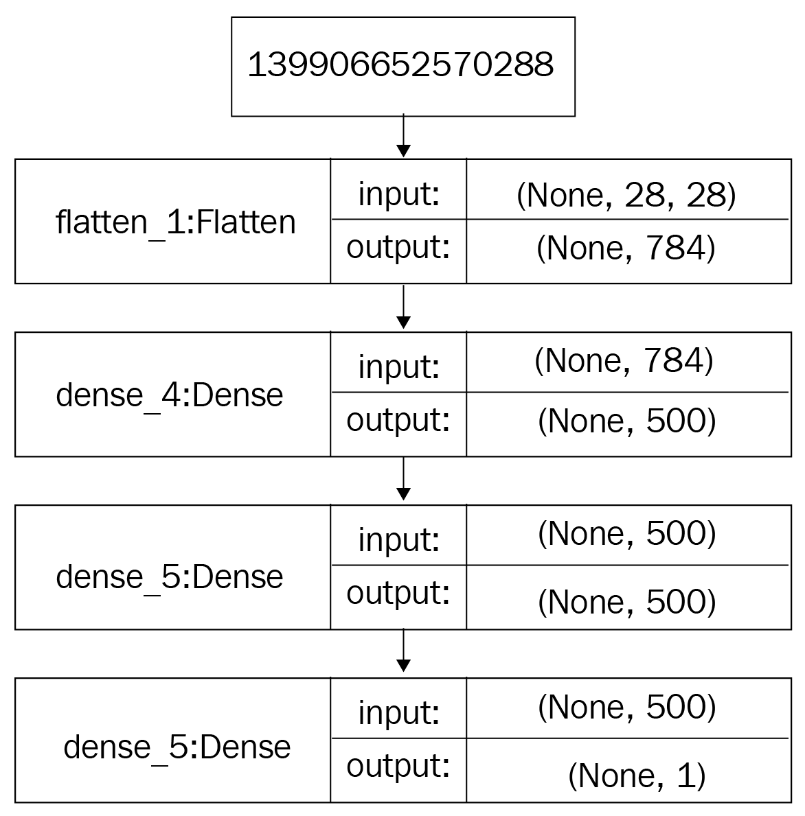
is the Kullback-Leibler divergence.

Now that we have learned about the KL divergence and the Jenson-Shannon divergence, let's discuss the Nash equilibrium for GANs.

Nash equilibrium

The Nash equilibrium describes a particular state in game theory. This state can be achieved in a non-cooperative game in which each player tries to pick the best possible strategy to gain the best possible outcome for themselves, based on what they expect the other players to do. Eventually, all the players reach a point at which they have all picked the best possible strategy for themselves based on the decisions made by the other players. At this point in the game, they would gain no benefit from changing their strategy. This state is the Nash equilibrium.

A famous example of how the Nash equilibrium can be reached is with the Prisoner's Dilemma. In this example, two criminals (A and B) have been arrested for committing a crime. Both have been placed in separate cells with no way of communicating with each other. The prosecutor only has enough evidence to convict them for a smaller offense and not the principal crime, which would see them go to jail for a long time. To get a conviction, the prosecutor gives them an offer:

  • If A and B both implicate each other in the principal crime, they both serve 2 years in jail.
  • If A implicates B but B remains silent, A will be set free and B will serve 3 years in jail (and vice versa).
  • If A and B both keep quiet, they both serve only 1 year in jail on the lesser charge.

From these three scenarios, it is obvious that the best possible outcome for A and B is to keep quiet and serve 1 year in jail. However, the risk of keeping quiet is 3 years as neither A nor B have any way of knowing that the other will also keep quiet. Thus, they would reach a state where their actual optimum strategy would be to confess as it is the choice that provides the highest reward and lowest penalty. When this state has been reached, neither criminal would gain any advantage by changing their strategy; thus, they would have reached a Nash equilibrium.

Objective functions

To create a generator network that generates images that are similar to real images, we try to increase the similarity of the data generated by the generator to real data. To measure the similarity, we use objective functions. Both networks have their own objective functions and during the training, they try to minimize their respective objective functions. The following equation represents the final objective function for GANs:

In the preceding equation, is the discriminator model, is the generator model, is the real data distribution, is the distribution of the data generated by the generator, and is the expected output.

During training, D (the Discriminator) wants to maximize the whole output and G (the Generator) wants to minimize it, thereby training a GAN to reach to an equilibrium between the generator and discriminator network. When it reaches an equilibrium, we say that the model has converged. This equilibrium is the Nash equilibrium. Once the training is complete, we get a generator model that is capable of generating realistic-looking images.

Scoring algorithms

Calculating the accuracy of a GAN is simple. The objective function for GANs is not a specific function, such as mean squared error or cross-entropy. GANs learn objective functions during training. There are many scoring algorithms proposed by researchers to measure how well a model fits. Let's look at some scoring algorithms in detail.

The inception score

The inception score is the most widely used scoring algorithm for GANs. It uses a pre-trained inception V3 network (trained on Imagenet) to extract the features of both generated and real images. It was proposed by Shane Barrat and Rishi Sharma in their paper, A Note on the Inception Score (https://arxiv.org/pdf/1801.01973.pdf). The inception score, or IS for short, measure the quality and the diversity of the generated images. Let's look at the equation for IS:

In the preceding equation, notation x represents a sample, sampled from a distribution. and represent the same concept. is the conditional class distribution, and is the marginal class distribution.

To calculate the inception score, perform the following steps:

  1. Start by sampling N number of images generated by the model, denoted as
  2. Then, construct the marginal class distribution, using the following equation:
  1. Then, calculate the KL divergence and the expected improvement, using the following equation:
  1. Finally, calculate the exponential of the result to give us the inception score.

The quality of the model is good if it has a high inception score. Even though this is an important measure, it has certain problems. For example, it shows a good level of accuracy even when the model generates one image per class, which means the model lacks diversity. To resolve this problem, other performance measures were proposed. We will look at one of these in the following section.

The Fréchet inception distance

To overcome the various shortcomings of the inception Score, the Fréchlet Inception Distance (FID) was proposed by Martin Heusel and others in their paper, GANs Trained by a Two Time-Scale Update Rule Converge to a Local Nash Equilibrium (https://arxiv.org/pdf/1706.08500.pdf).

The equation to calculate the FID score is as follows:

The preceding equation represents the FID score between the real images, x, and the generated images, g. To calculate the FID score, we use the Inception network to extract the feature maps from an intermediate layer in the Inception network. Then, we model a multivariate Gaussian distribution, which learns the distribution of the feature maps. This multivariate Gaussian distribution has a mean of and a covariance of , which we use to calculate the FID score. The lower the FID score, the better the model, and the more able it is to generate more diverse images with higher quality. A perfect generative model will have an FID score of zero. The advantage of using the FID score over the Inception score is that it is robust to noise and that it can easily measure the diversity of the images.

The TensorFlow implementation of FID can be found at the following link: https://www.tensorflow.org/api_docs/python/tf/contrib/gan/eval/frechet_classifier_distance
There are more scoring algorithms available that have been recently proposed by researchers in academia and industry. We won't be covering all of these here. Before reading any further, take a look at another scoring algorithm called the Mode Score, information about which can be found at the following link: https://arxiv.org/pdf/1612.02136.pdf.
Previous PageNext Page
You have been reading a chapter from
Generative Adversarial Networks Projects
Published in: Jan 2019Publisher: PacktISBN-13: 9781789136678
Register for a free Packt account to unlock a world of extra content!
A free Packt account unlocks extra newsletters, articles, discounted offers, and much more. Start advancing your knowledge today.
undefined
Unlock this book and the full library FREE for 7 days
Get unlimited access to 7000+ expert-authored eBooks and videos courses covering every tech area you can think of
Renews at $15.99/month. Cancel anytime

Author (1)

author image
Kailash Ahirwar

Kailash Ahirwar is a machine learning and deep learning enthusiast. He has worked in many areas of Artificial Intelligence (AI), ranging from natural language processing and computer vision to generative modeling using GANs. He is a co-founder and CTO of Mate Labs. He uses GANs to build different models, such as turning paintings into photos and controlling deep image synthesis with texture patches. He is super optimistic about AGI and believes that AI is going to be the workhorse of human evolution.
Read more about Kailash Ahirwar