RL in Discrete Optimization

Next, we will explore the new field in reinforcement learning (RL) application: discrete optimization problems, which will be showcased using the famous Rubik's Cube puzzle.

In this chapter, we will:

• Briefly discuss the basics of discrete optimization
• Cover step by step the paper called Solving the Rubik's Cube Without Human Knowledge, by UCI researchers Stephen McAleer et al., 2018, arxiv: 1805.07470, which applies RL methods to the Rubik's Cube optimization problem
• Explore experiments that I've done in an attempt to reproduce the paper's results and directions for future method improvement

RL's reputation

The perception of deep RL is that it is a tool to be used mostly for game playing. This is not surprising given the fact that, historically, the first success in the field was achieved on the Atari game suite by DeepMind in 2015 (https://deepmind.com/research/dqn/). The Atari benchmark suite (https://github.com/mgbellemare/Arcade-Learning-Environment) turned out to be very successful for RL problems and, even now, lots of research papers use it to demonstrate the efficiency of their methods. As the RL field progresses, the classic 53 Atari games continue to become less and less challenging (at the time of writing, almost all the games have been solved with superhuman accuracy) and researchers are turning to more complex games, like StarCraft and Dota 2.

This perception, which is especially prevalent in the media, is something that I've tried to counterbalance in this book by accompanying Atari games with examples from other domains, including stock trading...

The Rubik's Cube and combinatorial optimization

I doubt it's possible to find a person who hasn't heard about the Rubik's Cube, so I'm not going to repeat the Wikipedia description (https://en.wikipedia.org/wiki/Rubik%27s_Cube) of this puzzle, but rather focus on the connections it has to mathematics and computer science. If it's not explicitly stated, by "cube" I mean the 3×3 classic Rubik's Cube. There are lots of variations based on the original 3×3 puzzle, but they are still far less popular than the classic invention.

Despite being quite simple in terms of mechanics and the task at hand, the cube is quite a tricky object in terms of all the transformations we can make by possible rotations of its sides. It was calculated that in total, the cube has ~4.33 × 10¹⁹ distinct states reachable by rotating it. That's only the states that are reachable without disassembling the cube; by taking it apart and then assembling...

Optimality and God's number

What makes the combinatorial optimization problem tricky is that we're not looking for any solution; we're in fact interested in the optimal solution of the problem. The difference is obvious: right after the Rubik's Cube was invented, it was known how to reach the goal state (but it took Ernő Rubik about a month to figure out the first method of solving his own invention, which I guess was a frustrating experience). Nowadays, there are lots of different ways or schemes of cube solving: the beginner's method, the method by Jessica Fridrich (very popular among speedcubers), and so on.

All of them vary by the amount of moves to be taken. For example, a very simple beginner's method requires about 100 rotations to solve the cube using 5…7 sequences of rotations to be memorized. In contrast, the current world record in the speedcubing competition is solving the cube in 4.22 seconds, which requires much fewer steps...

Approaches to cube solving

Before the aforementioned paper was published, there were two major directions for solving the Rubik's Cube:

• By using group theory, it is possible to significantly reduce the state space to be checked. One of the most popular solutions using this approach is Kociemba's algorithm (https://en.wikipedia.org/wiki/Optimal_solutions_for_Rubik%27s_Cube#Kociemba's_algorithm).
• By using brute force search accompanied by manually crafted heuristics, we can direct the search in the most promising direction. A vivid example of this is Korf's algorithm (https://en.wikipedia.org/wiki/Optimal_solutions_for_Rubik%27s_Cube#Korf's_algorithm), which uses A* search with a large database of patterns to cut out bad directions.

The paper introduced a third approach: by training the neural network (NN) on lots of randomly shuffled cubes, it is possible to get the policy that will show us the direction to take toward the solved state. The...

The training process

Now that you know how the state of the cube is encoded in a 20 × 24 tensor, let's talk about the NN architecture and how it is trained.

The NN architecture

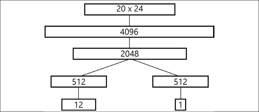
On the figure that follows (taken from the paper), the network architecture is shown.

Figure 24.2: The NN architecture transforming the observation (top) to the action and value (bottom)

As the input, it accepts the already familiar cube state representation as a 20 × 24 tensor and produces two outputs:

• The policy, which is a vector of 12 numbers, representing the probability distribution over our actions.
• The value, a single scalar estimating the "goodness" of the state passed. The concrete meaning of a value will be discussed later.

Between the input and output, the network has several fully connected layers with exponential linear unit (ELU) activations. In my implementation, the architecture is exactly the same as in the paper, and the model is...

The model application

Okay, imagine that we have trained the model using the process just described. How should we use it to solve the scrambled cube? From the network's structure, you might imagine the obvious, but not very successful, way:

1. Feed the model the current state of the cube that we want to solve
2. From the policy head, get the largest action to perform (or sample it from the resulting distribution)
3. Apply the action to the cube
4. Repeat the process until the solved state has been reached

On paper, this method should work, but in practice, it has one serious issue: it doesn't! The main reason for that is our model's quality. Due to the size of the state space and the nature of the NNs, it just isn't possible to train an NN to return the exact optimal action for any input state all of the time. Rather than telling us what to do to get the solved state, our model shows us promising directions to explore. Those directions could bring...

The paper's results

The final result published in the paper is quite impressive. After 44 hours of training on a machine with three GPUs, the network learned how to solve cubes at the same level as (and sometimes better than) human-crafted solvers. The final model has been compared against the two solvers described earlier: the Kociemba two-stage solver and Korf. The method proposed in the paper is named DeepCube.

To compare efficiency, 640 randomly scrambled cubes were used in all the methods. The depth of the scramble was 1,000 moves. The time limit for the solution was an hour and both the DeepCube and Kociemba solvers were able to solve all of the cubes within the limit. The Kociemba solver is very fast, and its median solution time is just one second, but due to the hardcoded rules implemented in the method, its solutions are not always the shortest ones.

The DeepCube method took much more time, with the median time being about 10 minutes, but it was able to match the...

The code outline

Okay, now let's switch to the code, which is in directory Chapter24 in the book's repository. In this section, I'm going to give a quick outline of my implementation and the key design decisions, but before that, I have to emphasize the important points about the code to set up the correct expectations:

• I'm not a researcher, so the original goal of this code was just to reimplement the paper's method. Unfortunately, the paper has very few details about the exact hyperparameters used, so I had to guess and experiment a lot, and still, my results are very different from those published in the paper.
• At the same time, I've tried to implement everything in a general way to simplify further experiments. For example, the exact details about the cube state and transformations are abstracted away, which allows us to implement more puzzles similar to the 3×3 cube just by adding a new module. In my code, two cubes are implemented...

The experiment results

Unfortunately, the paper provided no details about very important aspects of the method, like training hyperparameters, how deeply cubes were scrambled during the training, and the obtained convergence. To fill in the missing blanks, I did lots of experiments with various values of hyperparameters, but still my results are very different from those published in the paper. First of all, the training convergence of the original method is very unstable. Even with a small learning rate and a large batch size, the training eventually diverges, with the value loss component growing exponentially. Examples of this behavior are shown on the figure that follows.

Figure 24.5: The policy loss (left) and value loss (right) of two runs of the paper's method

After several experiments with this, I came to the conclusion that this behavior is a result of the wrong value objective being proposed in the method. Indeed, in the formula , the value returned by the...

Further improvements and experiments

There are lots of directions and things that could be tried:

• More input and network engineering: the cube is a complicated thing, so simple feed-forward NNs may not be the best model. Probably, the network could greatly benefit from convolutions.
• Oscillations and instability during training might be a sign of a common RL issue with inter-step correlations. The usual approach is the target network, when we use the old version of the network to get bootstrapped values.
• The priority replay buffer might help the training speed.
• My experiments show that the samples' weighting (inversely proportional to the scramble depth) helps to get a better policy that knows how to solve slightly scrambled cubes, but might slow down the learning of deeper states. Probably, this weighting could be made adaptive to make it less aggressive in later training stages.
• Entropy loss could be added to the training to regularize our policy.
...

Summary

In this chapter, I described the application of RL methods to discrete optimization problems, using the Rubik's Cube as a well-known, but still challenging, problem. In the final chapter of the book, we will talk about multi-agent problems in RL.