

Prediction using linear regression
Linear regression is one of the most widely known modeling techniques. Existing for more than 200 years, it has been explored from almost all possible angles. Linear regression assumes a linear relationship between the input variable (X) and the output variable (Y). The basic idea of linear regression is building a model, using training data that can predict the output given the input, such that the predicted output  is as near the observed training output Y for the input X. It involves finding a linear equation for the predicted value of the form:

where  are the n input variables, and
  are the linear coefficients, with b as the bias term. We can also expand the preceding equation to:

The bias term allows our regression model to provide an output even in the absence of any input; it provides us with an option to shift our data for a better fit. The error between the observed values (Y) and predicted values () for an input sample i is:

The goal is to find the best estimates for the coefficients W and bias b, such that the error between the observed values Y and the predicted values is minimized. Let’s go through some examples to better understand this.
Simple linear regression
If we consider only one independent variable and one dependent variable, what we get is a simple linear regression. Consider the case of house price prediction, defined in the preceding section; the area of the house (A) is the independent variable, and the price (Y) of the house is the dependent variable. We want to find a linear relationship between predicted price and A, of the form:

where b is the bias term. Thus, we need to determine W and b, such that the error between the price Y and the predicted price is minimized. The standard method used to estimate W and b is called the method of least squares, that is, we try to minimize the sum of the square of errors (S). For the preceding case, the expression becomes:

We want to estimate the regression coefficients, W and b, such that S is minimized. We use the fact that the derivative of a function is 0 at its minima to get these two equations:


These two equations can be solved to find the two unknowns. To do so, we first expand the summation in the second equation:

Take a look at the last term on the left-hand side; it just sums up a constant N time. Thus, we can rewrite it as:

Reordering the terms, we get:

The two terms on the right-hand side can be replaced by  , the average price (output), and
  , the average area (input), respectively, and thus we get:

In a similar fashion, we expand the partial differential equation of S with respect to weight W:

Substitute the expression for the bias term b:

Reordering the equation:

Playing around with the mean definition, we can get from this the value of weight W as:

where and are the average price and area, respectively. Let us try this on some simple sample data:
- We import the necessary modules. It is a simple example, so we’ll be using only NumPy, pandas, and Matplotlib:
import tensorflow as tf import numpy as np import matplotlib.pyplot as plt import pandas as pd - Next, we generate random data with a linear relationship. To make it more realistic, we also add a random noise element. You can see the two variables (the cause,
area, and the effect,price) follow a positive linear dependence:#Generate a random data np.random.seed(0) area = 2.5 * np.random.randn(100) + 25 price = 25 * area + 5 + np.random.randint(20,50, size = len(area)) data = np.array([area, price]) data = pd.DataFrame(data = data.T, columns=['area','price']) plt.scatter(data['area'], data['price']) plt.show()
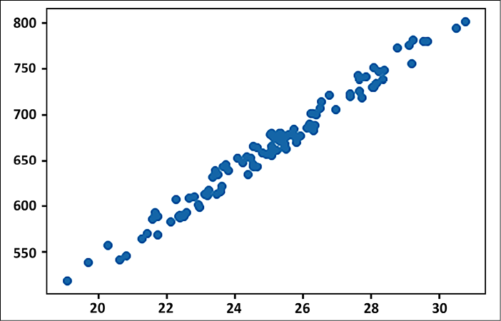
Figure 2.1: Scatter plot between the area of the house and its price
- Now, we calculate the two regression coefficients using the equations we defined. You can see the result is very much near the linear relationship we have simulated:
W = sum(price*(area-np.mean(area))) / sum((area-np.mean(area))**2)
b = np.mean(price) - W*np.mean(area)
print("The regression coefficients are", W,b)
----------------------------------------------- The regression coefficients are 24.815544052284988 43.4989785533412 - Let us now try predicting the new prices using the obtained weight and bias values:
y_pred = W * area + b - Next, we plot the predicted prices along with the actual price. You can see that predicted prices follow a linear relationship with the area:
plt.plot(area, y_pred, color='red',label="Predicted Price")
plt.scatter(data['area'], data['price'], label="Training Data")
plt.xlabel("Area")
plt.ylabel("Price")
plt.legend()
Figure 2.2: Predicted values vs the actual price
From Figure 2.2, we can see that the predicted values follow the same trend as the actual house prices.
Multiple linear regression
The preceding example was simple, but that is rarely the case. In most problems, the dependent variables depend upon multiple independent variables. Multiple linear regression finds a linear relationship between the many independent input variables (X) and the dependent output variable (Y), such that they satisfy the predicted Y value of the form:
where  are the n independent input variables, and are the linear coefficients, with b as the bias term.
As before, the linear coefficients Ws are estimated using the method of least squares, that is, minimizing the sum of squared differences between predicted values () and observed values (Y). Thus, we try to minimize the loss function (also called squared error, and if we divide by n, it is the mean squared error):

where the sum is over all the training samples.
As you might have guessed, now, instead of two, we will have n+1 equations, which we will need to simultaneously solve. An easier alternative will be to use the TensorFlow Keras API. We will learn shortly how to use the TensorFlow Keras API to perform the task of regression.
Multivariate linear regression
There can be cases where the independent variables affect more than one dependent variable. For example, consider the case where we want to predict a rocket’s speed and its carbon dioxide emission – these two will now be our dependent variables, and both will be affected by the sensors reading the fuel amount, engine type, rocket body, and so on. This is a case of multivariate linear regression. Mathematically, a multivariate regression model can be represented as:

where  and
and  . The term
  represents the jth predicted output value corresponding to the ith input sample, w represents the regression coefficients, and xik is the kth feature of the ith input sample. The number of equations needed to solve in this case will now be n x m. While we can solve these equations using matrices, the process will be computationally expensive as it will involve calculating the inverse and determinants. An easier way would be to use the gradient descent with the sum of least square error as the loss function and to use one of the many optimizers that the TensorFlow API includes.
In the next section, we will delve deeper into the TensorFlow Keras API, a versatile higher-level API to develop your model with ease.