The learning process of a neural network is configured as an iterative process of optimization of the weights, and is therefore of the supervised type. The weights are modified based on the network performance on a set of examples belonging to the training set, where the category they belong to is known. The aim is to minimize a loss function, which indicates the degree to which the behavior of the network deviates from the desired one. The performance of the network is then verified on a test set consisting of objects (for example, images in a image classification problem) other than those of the training set.
How does an artificial neural network learn?
The backpropagation algorithm
A supervised learning algorithm used is the backpropagation algorithm.
The basic steps of the training procedure are as follows:
- Initialize the net with random weights.
- For all training cases:
- Forward pass: Calculates the error committed by the net, the difference between the desired output and the actual output.
- Backward pass: For all layers, starting with the output layer, back to the input layer.
- Show the network layer output with correct input (error function).
- Adapt weights in the current layer to minimize the error function. This is the backpropagation's optimization step. The training process ends when the error on the validation set begins to increase, because this could mark the beginning of a phase of over-fitting of the network, that is, the phase in which the network tends to interpolate the training data at the expense of generalization ability.
Weights optimization
The availability of efficient algorithms to weights optimization, therefore, constitutes an essential tool for the construction of neural networks. The problem can be solved with an iterative numerical technique called gradient descent (GD).
This technique works according to the following algorithm:
- Some initial values for the parameters of the model are chosen randomly.
- Compute the gradient G of the error function with respect to each parameter of the model.
- Change the model's parameters so that they move in the direction of decreasing the error, that is, in the direction of -G.
- Repeat steps 2 and 3 until the value of G approaches zero.
In mathematics, the gradient of a scalar field is a real-valued function of several variables, then defined in a region of a space in two, three, or more dimensions. The gradient of a function is defined as the vector that has Cartesian components for the partial derivatives of the function. The gradient represents the direction of maximum increment of a function of n variables: f (x1, x2,...., xn). The gradient is then a vector quantity that indicates a physical quantity as a function of its various different parameters.
The gradient G of the error function E provides the direction in which the error function with the current values has the steeper slope, so to decrease E, we have to make some small steps in the opposite direction, -G (see the following figures).
By repeating this operation several times in an iterative manner, we move in the direction in which the gradient G of the function E is minimal (see the following figure):
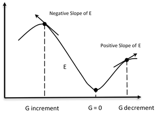
Figure 6: Gradient descent procedure
As you can see, we move in the direction in which the gradient G of the function E is minimal.
Stochastic gradient descent
In GD optimization, we compute the cost gradient based on the complete training set; hence, we sometimes also call it batch GD. In the case of very large datasets, using GD can be quite costly, since we are only taking a single step for one pass over the training set. Thus, the larger the training set, the slower our algorithm updates the weights and the longer it may take until it converges to the global cost minimum.
An alternative approach and the fastest of gradient descent, and for this reason, used in DNNs, is the Stochastic Gradient Descent (SGD).
In SGD, we use only one training sample from the training set to do the update for a parameter in a particular iteration. Here, the term stochastic comes from the fact that the gradient based on a single training sample is a stochastic approximation of the true cost gradient.
Due to its stochastic nature, the path toward the global cost minimum is not direct, as in GD, but may zigzag if we are visualizing the cost surface in a 2D space (see the following figure, (b) Stochastic Gradient Descent - SDG).
We can make a comparison between these optimization procedures, showing the next figure, the gradient descent (see the following figure, (a) Gradient Descent - GD) assures that each update in the weights is done in the right direction--the one that minimizes the cost function. With the growth of datasets' size, and more complex computations in each step, SGD came to be preferred in these cases. Here, updates to the weights are done as each sample is processed and, as such, subsequent calculations already use improved weights. Nonetheless, this very reason leads to it incurring some misdirection in minimizing the error function:
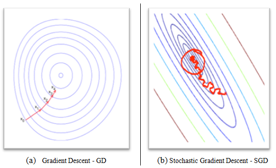
Figure 7: GD versus SDG