


Combining data in SQL – the JOIN clause
The JOIN clause, and the equivalent forms of the FROM clause with multiple tables, is used to combine the rows from two tables to create a row with the columns (that you select) from both tables.
Joins are useful when the tables to be combined are related, that is, when the two tables have some columns that represent the same thing, and we want to combine data from both tables.
We express how to combine the rows by providing a join clause, usually with the ON subclause, which compares the rows from one table to the rows of the other table. Most of the time, the relation is that the values of corresponding columns are the same, but any predicate is fine in the ON subclause.
Combining orders and customers
One example of how to combine data might be a web_order table and a customer table.
In both tables, you normally have a column with the customer ID information even if the columns might not have the same name. Let’s assume that in the order table, there is the ID of the customer who placed the order in the ORDER_PLACED_BY column, and in the customer table, there is the ID of the customer in the CUSTOMER_ID column. Then, we could write the following query:
SELECT *
FROM web_order
JOIN customer ON ORDER_PLACED_BY = CUSTOMER_ID;
This query, using *, returns rows that have all columns from both tables, in all the cases when there is a row that satisfies the ON condition.
Let’s look at the relevant rows of the input and output tables in the case where we have one order with ORDER_PLACED_BY = 123 in the order table and one customer with CUSTOMER_ID = 123.
Say we have one row with ORDER_PLACED_BY = 123 in the web_order table, as follows:
|
Order_ID |
ORDER_PLACED_BY |
ORDER_VALUE |
|
WEB_0001 |
123 |
225.52 |
Table 1.2: Sample web_order table
And we have one row with CUSTOMER_ID = 123 in the customer table, as follows:
|
Customer_ID |
Customer_Name |
Address |
|
123 |
Big Buyer LLP |
Nice place road, 00100 SOMEWHERE |
Table 1.3: Sample customer table
Then, we get the following row in the result table:
|
Order_ID |
ORDER_PLACED_BY |
ORDER_VALUE |
Customer_ID |
Customer_Name |
Address |
|
WEB_0001 |
123 |
225.52 |
123 |
Big Buyer LLP |
Nice … |
Table 1.4: Sample result of the previous query
If we do not have any customer with CUSTOMER_ID = 123, then we will have no row returned (for that order) in the result table.
Say we have the same order table as before, but three rows with CUSTOMER_ID = 123 in the customer table:
|
Customer_ID |
Customer_Name |
Address |
|
123 |
Big Buyer LLP |
Nice place road, 00100 SOMEWHERE |
|
123 |
Another Customer |
Some road, 10250 SOME PLACE |
|
123 |
A third customer |
No way road, 20100 NOWHERE |
Table 1.5: Alternative example of a customer table with three rows with CUSTOMER_ID = 123
Then, we will have three rows returned, each having the same order information combined with one specific customer per row, as you see in the following table:
|
Order_ID |
ORDER_PLACED_BY |
ORDER_VALUE |
Customer_ID |
Customer_Name |
Address |
|
WEB_0001 |
123 |
225.52 |
123 |
Big Buyer LLP |
Nice … |
|
WEB_0001 |
123 |
225.52 |
123 |
Another Customer |
Some … |
|
WEB_0001 |
123 |
225.52 |
123 |
A third customer |
No … |
Table 1.6: Table resulting from the previous sample JOIN query, with three customer matches
This last situation is probably not what you want, as it will “duplicate” the order, returning one row with the same order information for each customer that matches the condition. Later in the book, when we talk about identity, we will see how to make sure that this does not happen and how with dbt, you can also easily test that it really does not happen.
Another question that you might have is how do we keep the order information in the results, even if we do not have a match in the customer table, so that we get all the orders, with the customer information when available? That’s a good question, and the next topic on join types will enlighten you.
JOIN types
In the previous section about the query syntax, we introduced the simplified syntax of a JOIN clause. Let’s recall it here with shorter table names and no aliases:
SELECT …
FROM t1
[<join type>] JOIN t2 ON <condition_A>
[[<join type>] JOIN t3 ON <condition_B>]
…
In the most common cases, the join type is one of [INNER] or { LEFT | RIGHT | FULL } [ OUTER ].
This gives us the following possible joins with a join condition using the ON subclause:
INNER JOIN: This is the default and most common type of join, returning only the rows that have a match on the join condition. TheINNERkeyword is optional, so you can write the following:SELECT … FROM t1 JOIN t2 ON <some condition>
Note that the preceding INNER JOIN is equivalent to the following query that uses only FROM and WHERE:
SELECT … FROM t1, t2 WHERE <some condition>
It is preferable, anyway, to use the JOIN syntax, which clearly shows, especially to humans, which conditions are for the join and which are for filtering the incoming data.
LEFT OUTER JOIN: This is the second most used type of join, as it returns all the rows from the left table, which is the first to be named, combined with the matching rows from the other table, padding withNULLthe values where the right table has no matches
Of course, you will have one row of the left table for each matching row of the right table.
RIGHT OUTER JOIN: This is similar toLEFT OUTER JOIN, but it keeps all the columns from the right table and the matching ones from the left table. It is less used than the left as you can reverse the table order and use the left expression.
The query t1 RIGHT OUTER JOIN t2 is the same as t2 LEFT OUTER JOIN t1.
FULL OUTER JOIN: This type of join combines the left and right behavior to keep all the rows from left and right, padding with nulls the columns where there is no match.
There are also two other types of join where you do not specify a join condition:
CROSS JOIN: This type of join produces a Cartesian product, with all possible combinations of rows from both tables. This is also what you obtain if you do not use anONsubclause when using the previous types of joins. The cross join does not have anONsubclause:SELECT … FROM t1 CROSS JOIN t2
This is equivalent to what we have seen in the FROM clause:
SELECT … FROM t1, t2
The difference is just how obvious it is for a human reader that you really want to have a cross join, or that you forgot about the ON subclause or some join-related condition in the WHERE clause. It is not so common to use cross joins, because of the Cartesian explosion we talked about; it is, therefore, a much better style to explicitly indicate that you really want a cross join, the few times when you will actually want it.
NATURAL <type> JOIN: TheNATURALjoin is identical to the various types ofJOINs that we have seen so far, but instead of using theONsubclause to find the matches between the two tables, it uses the columns that have the same name with an equality condition. Another small difference is that the columns with the same name in the two tables are returned only once in the results as they always have the same values on both sides, because of the equality condition.
Here are a couple of examples of how to write queries with this type of join:
SELECT … FROM t1 NATURAL INNER JOIN t2
The preceding query is like an INNER JOIN query on columns with the same name in t1 and t2.
SELECT … FROM t1 NATURAL FULL OUTER JOIN t2
This one is like a FULL OUTER JOIN query on columns with the same name in t1 and t2.
Tip
When talking about JOIN, we use LEFT and RIGHT, but with respect to what?
It is a reference to the order in which the tables appear in a chain of joins.
The FROM table is the leftmost one and any other table that is joined is added to the right in the order in which the join appears.
Writing SELECT … FROM t1 JOIN t2 ON … JOIN t3 ON … JOIN t4 ON … makes clear that the tables will be stacked from left to right like this: t1-t2-t3-t4.
You could rewrite the same example as it is normally written on multiple lines, as follows:
SELECT …
FROM t1
JOIN t2 ON …
JOIN t3 ON …
JOIN t4 ON …
The result is the same, even if it is not so immediate to see left and right as mentioned in the previous statement.
Visual representation of join types
We have defined how joins work through examples and explanations, but I think that for some people, an image is worth a thousand explanations, so I propose two ways to graphically look at joins:
- One that tries to show how the matching and non-matching rows are treated in different kinds of joins
- One that uses a set notation and compares the different types of joins
Visual representation of returned rows in JOIN queries
The following figure visually describes how two rows of tables A and B are aligned to form the rows resulting from the different types of joins:
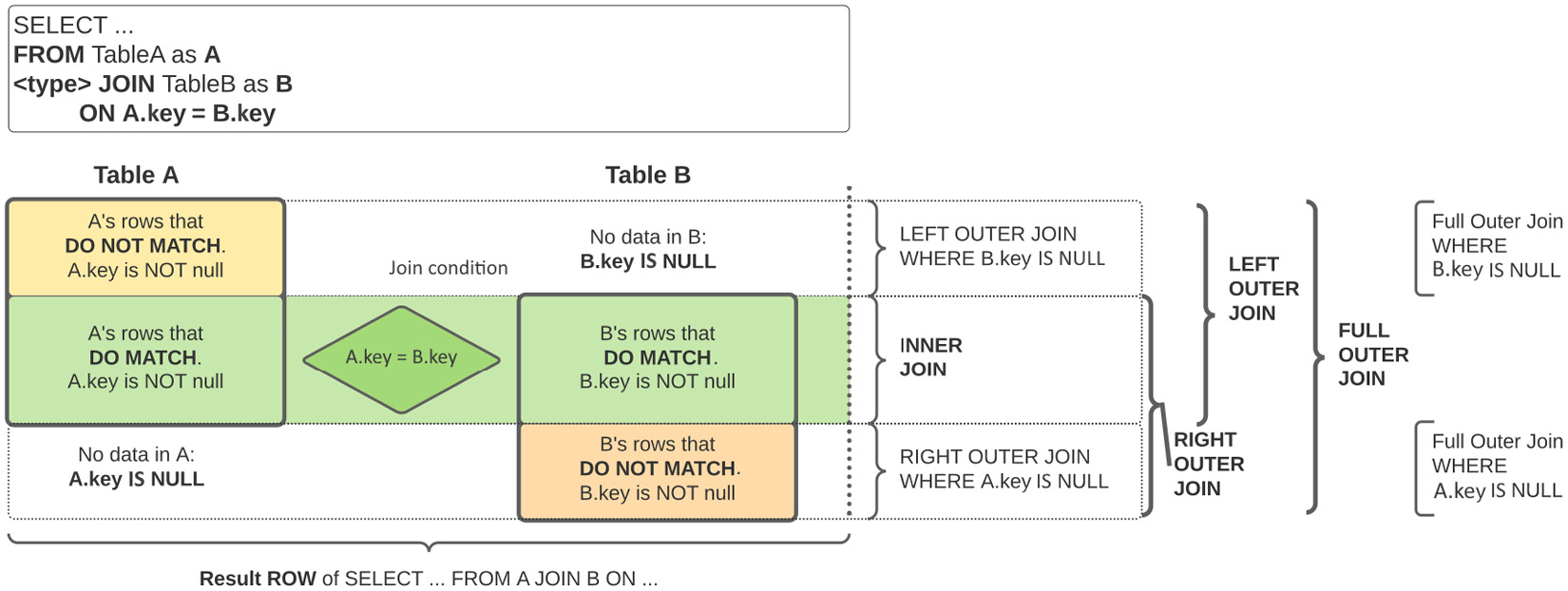
Figure 1.7: Visual representation of different JOIN types between tables A and B
Each table is divided into two: one part where the rows have one or more matches on the other table that satisfy the join condition and another part where each row has no match on the other table.
The rows from the two tables that have a match, in the center of the figure, are properly aligned according to the matching condition so that each resulting row contains the values from A’s columns and B’s columns where the condition is met. This central part is always returned by all joins, unless explicitly excluded with a WHERE clause requesting one of the two keys to be NULL.
The rows where there is no match, shown at the top for table A and at the bottom for table B, are aligned with columns from the other table padded with NULL values. This produces the somewhat unintuitive result that a query with an ON A.key = B.key clause might produce rows where one of the two keys is NULL and the other is not.
Tip
Please remember that NULL is a special value and not all things work out as expected. As an example, the expression NULL = NULL produces NULL and not TRUE as you might expect.
Try it out yourself with this query: SELECT NULL = NULL as unexpected;.
That is why you test for NULL values using <field> IS NULL and not using equality.
Full outer join
The following figure depicts the result of a FULL OUTER JOIN in terms of the rows of the two original tables:
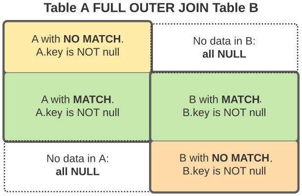
Figure 1.8: Visual representation of a FULL OUTER JOIN
You can clearly identify the central part of the previous picture, where rows from both tables satisfy the join constraint and the two parts where one of the tables has no matching rows for the other table; in these rows, the columns from the other table are filled with NULL values.
Left outer join
The following figure depicts the result of a LEFT OUTER JOIN in terms of the rows from the two original tables:
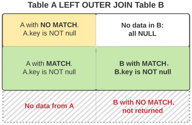
Figure 1.9: Visual representation of a LEFT OUTER JOIN
You can clearly see in the picture that the result consists of the rows from both sides that satisfy the join constraints, plus only the rows from table A that do not have a match in table B, with the columns from B filled with NULL values.
The rows from table B without a match in table A are not returned.
Another way to express this is that we have all rows from table A, plus the rows from B where there is a match in the join condition, and NULL for the other rows.
Important Note
When we join two tables, and we write a condition such as ON A.key = B.key, we are expressing interest in rows where this condition is true, and INNER JOIN just gives us these rows.
However, OUTER joins also return rows where the join clause is not true; in these rows, either the A.key or B.key column will be filled with NULL as there is no match on the other table.
Visual representation of JOIN results using sets
The following figure visually represents the join types that use an ON clause, representing, as sets, the rows from tables A and B that match or do not match the join condition in the ON clause.
The overlapping area is where the condition is matched by rows in both tables:
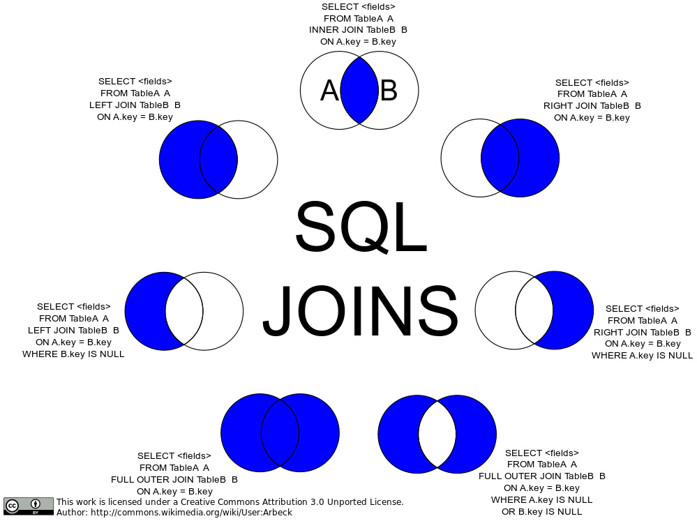
Figure 1.10: Visual representation of SQL JOIN types with an ON clause, as set operations
The preceding figure represents the join types that we have seen in two forms:
- Using only the
ONsubclause, showing the results of the pure join - Using a
WHEREclause on the column used in theONsubclause
In the figure, this information is used to exclude from the outer joins the rows where the match happens, where A and B overlap, which are the rows returned by an inner join.
This type of query is useful, and often used, for example, to see whether we have orders where the referenced customer does not exist in the customer table. This would be called an orphan key in the order table.
Let’s see an example using Snowflake sample data:
SELECT *
FROM "SNOWFLAKE_SAMPLE_DATA"."TPCH_SF1"."ORDERS"
LEFT OUTER JOIN "SNOWFLAKE_SAMPLE_DATA"."TPCH_SF1"."CUSTOMER"
  ON C_CUSTKEY = O_CUSTKEY
WHERE C_CUSTKEY is NULL;
This query should return no rows, as all the customers referenced by the orders should exist in the customer table. Now that we have covered all the basic functions in SQL, let us check out an advanced feature: windows functions.


