You're reading from A Practical Guide to Quantum Machine Learning and Quantum Optimization

Product typeBook

Published inMar 2023

PublisherPackt

ISBN-139781804613832

Edition1st Edition

Concepts

Quantum Computing

Authors (2):

Elías F. Combarro

Samuel González-Castillo

View More author details

1.3 Working with one qubit and the Bloch sphere

One of the advantages of using a computational model is that you can forget about the particularities of the physical implementation of your computer and focus instead on the properties of the elements on which you store information and the operations you can perform on them. For instance, we could define a qubit as a (physical) quantum system that is capable of being in two different states. In practice, it could be a photon with two possible polarizations, a particle with two possible values for its spin, or a superconducting circuit, whose current can be flowing in one of two directions. When using the quantum circuit model, we can forget about those implementation details and just define a qubit…as a mathematical vector!

1.3.1 What is a qubit?

In fact, a qubit (short for quantum bit, sometimes also written as qbit, Qbit or even q-bit) is the minimal information unit in quantum computing. In the same way that a bit (short for binary digit) can be in state or in state , a qubit can be in state $\left| 0 \right\rangle$ or in state $\left| 1 \right\rangle$ . Here, we are using the so-called Dirac notation, where these funny-looking symbols surrounding and are called kets and are used to indicate that we are dealing with vectors instead of regular numbers. In fact, $\left| 0 \right\rangle$ and $\left| 1 \right\rangle$ are not the only possibilities for the state of a qubit and, in general, it could be in a superposition of the form

$a\left| 0 \right\rangle + b\left| 1 \right\rangle,$

where and are complex numbers, called amplitudes, such that $|a|^{2} + |b|^{2} = 1$ . The quantity $\sqrt{|a|^{2} + |b|^{2}}$ is called the norm or length of the state and, when it is equal to , we say that the state is normalized.

To learn more…

If you need a refresher on complex numbers or vector spaces, please check Appendix A, Complex Numbers, and Appendix B, Basic Linear Algebra.

All these possible values for the state of a single qubit are vectors that live in a complex vector space of dimension 2 (in fact, they live in what is called a Hilbert space, but since we will be working only with finite dimensions, there is no real difference). Thus we shall fix the vectors $\left| 0 \right\rangle$ and $\left| 1 \right\rangle$ as elements of a special basis, which we will refer to as the computational basis. We will represent these vectors, constituents of the computational basis, as the column vectors

$\left| 0 \right\rangle = \begin{pmatrix} 1 \\ 0 \\ \end{pmatrix},\qquad\left| 1 \right\rangle = \begin{pmatrix} 0 \\ 1 \\ \end{pmatrix}$

and hence

$a\left| 0 \right\rangle + b\left| 1 \right\rangle = a\begin{pmatrix} 1 \\ 0 \\ \end{pmatrix} + b\begin{pmatrix} 0 \\ 1 \\ \end{pmatrix} = \begin{pmatrix} a \\ b \\ \end{pmatrix}.$

If we are given a qubit and we want to determine or, rather, estimate its state, all we can do is perform a measurement and get one of two possible results: 0 or 1. We have nonetheless seen how a qubit can be in infinitely many states, so how does the state of a qubit determine the outcome of a measurement? As you likely already know, in quantum physics, these measurements are not deterministic, but probabilistic. In particular, given any qubit $a\left| 0 \right\rangle + b\left| 1 \right\rangle$ , the probability of getting upon a measurement is $|a|^{2}$ , while that of getting is $|b|^{2}$ . Naturally, these two probabilities must add up to 1, hence the need for the normalization condition $|a|^{2} + |b|^{2} = 1$ .

If upon measuring a qubit we get, let's say, , we then know that, after the measurement, the state of the qubit is $\left| 0 \right\rangle$ , and we say that the qubit has collapsed into that state. If we obtain , the state collapses to $\left| 1 \right\rangle$ . Since we are obtaining results that correspond to $\left| 0 \right\rangle$ and $\left| 1 \right\rangle$ , we say that we are measuring in the computational basis.

Exercise 1.1

What is the probability of measuring 0 if the state of a qubit is $\sqrt{\left. 1\slash 2 \right.}\left| 0 \right\rangle + \sqrt{\left. 1\slash 2 \right.}\left| 1 \right\rangle$ ? And the probability of measuring 1? What if the state of the qubit is $\sqrt{\left. 1\slash 3 \right.}\left| 0 \right\rangle + \sqrt{\left. 2\slash 3 \right.}\left| 1 \right\rangle$ ? And if it is $\sqrt{\left. 1\slash 2 \right.}\left| 0 \right\rangle - \sqrt{\left. 1\slash 2 \right.}\left| 1 \right\rangle$ ?

So a qubit is, mathematically, just a 2-dimensional vector that satisfies a normalization condition. Who could have known? But the surprises do not end here. In the next subsection, we will see how we can use those funny-looking kets to compute inner products in a very easy way.

1.3.2 Dirac notation and inner products

Dirac notation can not only be used for column vectors, but also for row vectors. In that case, we talk of bras, which, together with kets, can be used to form bra-kets. This name is a pun, because, as we are about to show, bra-kets are, in fact, inner products that are written — you guessed it — between brackets. To be more mathematically precise, with each ket we can associate a bra that is its adjoint or conjugate transpose or Hermitian transpose. In order to obtain this adjoint, we take the ket's column vector, we transpose it and conjugate each of its coordinates (which are, as we already know, complex numbers). We use $\left\langle 0 \right|$ to denote the bra associated with $\left| 0 \right\rangle$ and $\left\langle 1 \right|$ to denote the bra associated with $\left| 1 \right\rangle$ , so we have

$\left\langle 0 \right| = \left| 0 \right\rangle^{\dagger} = \begin{pmatrix} 1 \\ 0 \\ \end{pmatrix}^{\dagger} = \begin{pmatrix} 1 & 0 \\ \end{pmatrix},\qquad\left\langle 1 \right| = \left| 1 \right\rangle^{\dagger} = \begin{pmatrix} 0 \\ 1 \\ \end{pmatrix}^{\dagger} = \begin{pmatrix} 0 & 1 \\ \end{pmatrix}$

and, in general,

$a\left\langle 0 \right| + b\left\langle 1 \right| = a\left| 0 \right\rangle^{\dagger} + b\left| 1 \right\rangle^{\dagger} = a\begin{pmatrix} 1 & 0 \\ \end{pmatrix} + b\begin{pmatrix} 0 & 1 \\ \end{pmatrix} = \begin{pmatrix} a & b \\ \end{pmatrix},$

where, as it is customary, we use the dagger symbol ( $\dagger$ ) for the adjoint.

Important note

When finding the adjoint, do not forget to conjugate the complex numbers! For instance, it holds that

$\begin{pmatrix} \frac{1 - i}{2} \\ \frac{i}{\sqrt{2}} \\ \end{pmatrix}^{\dagger} = \begin{pmatrix} \frac{1 + i}{2} & \frac{- i}{\sqrt{2}} \\ \end{pmatrix}.$

One of the reasons why Dirac notation is so popular for working with quantum systems is that, by using it, we can easily compute the inner products of kets and bras. For instance, we can readily show that

$\left\langle 0 \middle| 0 \right\rangle = \begin{pmatrix} 1 & 0 \\ \end{pmatrix}\begin{pmatrix} 1 \\ 0 \\ \end{pmatrix} = 1,\qquad\left\langle 0 \middle| 1 \right\rangle = \begin{pmatrix} 1 & 0 \\ \end{pmatrix}\begin{pmatrix} 0 \\ 1 \\ \end{pmatrix} = 0,$

$\left\langle 1 \middle| 0 \right\rangle = \begin{pmatrix} 0 & 1 \\ \end{pmatrix}\begin{pmatrix} 1 \\ 0 \\ \end{pmatrix} = 0,\qquad\left\langle 1 \middle| 1 \right\rangle = \begin{pmatrix} 0 & 1 \\ \end{pmatrix}\begin{pmatrix} 0 \\ 1 \\ \end{pmatrix} = 1.$

This proves that $\left| 0 \right\rangle$ and $\left| 1 \right\rangle$ are not just elements of any basis but of an orthonormal one, since $\left| 0 \right\rangle$ and $\left| 1 \right\rangle$ are orthogonal and of length 1. Thus, we can compute the inner product of two states $\left| \psi_{1} \right\rangle = a\left| 0 \right\rangle + b\left| 1 \right\rangle$ and $\left| \psi_{2} \right\rangle = c\left| 0 \right\rangle + d\left| 1 \right\rangle$ using Dirac notation by noting that

$\begin{array}{rlrl} \left\langle \psi_{1} \middle| \psi_{2} \right\rangle & {= \left( {a^{\ast}\left\langle 0 \right| + b^{\ast}\left\langle 1 \right|} \right)\left( {c\left| 0 \right\rangle + d\left| 1 \right\rangle} \right)\qquad} & & \qquad \\ & {= a^{\ast}c\left\langle 0 \middle| 0 \right\rangle + a^{\ast}d\left\langle 0 \middle| 1 \right\rangle + b^{\ast}c\left\langle 1 \middle| 0 \right\rangle + b^{\ast}d\left\langle 1 \middle| 1 \right\rangle\qquad} & & \qquad \\ & {= a^{\ast}c + b^{\ast}d,\qquad} & & \qquad \\ \end{array}$

where $a^{\ast}$ and $b^{\ast}$ are the complex conjugates of and .

Exercise 1.2

What is the inner product of $\sqrt{\left. 1\slash 2 \right.}\left| 0 \right\rangle + \sqrt{\left. 1\slash 2 \right.}\left| 1 \right\rangle$ and $\sqrt{\left. 1\slash 3 \right.}\left| 0 \right\rangle + \sqrt{\left. 2\slash 3 \right.}\left| 1 \right\rangle$ ? And the inner product of $\sqrt{\left. 1\slash 2 \right.}\left| 0 \right\rangle + \sqrt{\left. 1\slash 2 \right.}\left| 1 \right\rangle$ and $\sqrt{\left. 1\slash 2 \right.}\left| 0 \right\rangle - \sqrt{\left. 1\slash 2 \right.}\left| 1 \right\rangle$ ?

To learn more…

Notice that, if $\left| \psi \right\rangle = a\left| 0 \right\rangle + b\left| 1 \right\rangle$ , then $\left| \left\langle 0 \middle| \psi \right\rangle \right|^{2} = |a|^{2}$ , which is the probability of measuring if the state is $\left| \psi \right\rangle$ . This is not accidental. In Chapter 7, VQE: Variational Quantum Eigensolver, for example, we will use measurements in orthonormal bases other than the computational one, and we will see how, in that case, the probability of measuring the result associated to an element $\left| \varphi \right\rangle$ of a given orthonormal basis is exactly $\left| \left\langle \varphi \middle| \psi \right\rangle \right|^{2}$ .

We now know what qubits are, how to measure them, and even how to benefit from Dirac notation for some useful computations. The only thing remaining is to study how to operate on qubits. Are you ready? It is time for us to get you introduced to the mighty quantum gates!

1.3.3 One-qubit quantum gates

So far, we have focused on how a qubit stores information in its state and on how we can access (part of) that information with measurements. But in order to develop useful algorithms, we also need some way of manipulating the state of qubits to perform computations.

Since a qubit is, fundamentally, a quantum system, its evolution follows the laws of quantum mechanics. More precisely, if we suppose that our system is isolated from its environment, it obeys the famous Schrödinger equation.

To learn more…

The time-independent Schrödinger equation can be written as

$H\left| {\psi(t)} \right\rangle = i\hslash\frac{\partial}{\partial t}\left| {\psi(t)} \right\rangle,$

where is the Hamiltonian of the system, $\left| {\psi(t)} \right\rangle$ is the state vector of the system at time , is the imaginary unit, and $\hslash$ is the reduced Planck constant.

We will talk more about Hamiltonians in Chapter 3, QUBO: Quadratic Unconstrained Binary Optimization, Chapter 4, Quantum Adiabatic Computing and Quantum Annealing, and Chapter 7, VQE: Variational Quantum Eigensolver.

Don't panic! To program a quantum computer, you don't need to know how to solve Schrödinger's equation. In fact, the only thing that you need to know is that its solutions are always a special type of linear transformations. For the purposes of the quantum circuit model, since we are working in finite-dimensional spaces and we have fixed a basis, the operations can be described by matrices that are applied to the vectors that represent the states of the qubits.

But not any kind of matrix does the trick. According to quantum mechanics, the only matrices that we can use are the so-called unitary matrices, which are the matrices such that

$U^{\dagger}U = UU^{\dagger} = I,$

where is the identity matrix and $U^{\dagger}$ is the adjoint of , that is, the matrix obtained by transposing and replacing each element by its complex conjugate. This means that any unitary matrix is invertible and its inverse is given by $U^{\dagger}$ . In the context of the quantum circuit model, the operations represented by these matrices are called quantum gates.

To learn more…

It is relatively easy to check that unitary matrices preserve vector lengths (see, for instance, Section 5.7.5 in Dancing with Qubits, by Robert Sutor [92]). That is, if is a unitary matrix and $\left| \psi \right\rangle$ is a quantum state (and, hence, its norm is , as we already know) then $U\left| \psi \right\rangle$ also is a valid quantum state because its norm is still . For this reason, we can safely apply unitary matrices to our quantum states and rest assured that the resulting states will satisfy the normalization condition.

When we have just one qubit, our unitary matrices need to be of size $2 \times 2$ because the state vector is of dimension 2. Thus, the simplest example of a quantum gate is the identity matrix of dimension 2, which transforms the state of the qubit by... well, by not transforming it at all. A less boring example is the gate, whose matrix is given by

$X = \begin{pmatrix} 0 & 1 \\ 1 & 0 \\ \end{pmatrix}.$

The gate is also called the NOT gate, because its action on the elements of the computational basis is

$X\left| 0 \right\rangle = \begin{pmatrix} 0 & 1 \\ 1 & 0 \\ \end{pmatrix}\begin{pmatrix} 1 \\ 0 \\ \end{pmatrix} = \begin{pmatrix} 0 \\ 1 \\ \end{pmatrix} = \left| 1 \right\rangle,\qquad X\left| 1 \right\rangle = \begin{pmatrix} 0 & 1 \\ 1 & 0 \\ \end{pmatrix}\begin{pmatrix} 0 \\ 1 \\ \end{pmatrix} = \begin{pmatrix} 1 \\ 0 \\ \end{pmatrix} = \left| 0 \right\rangle,$

which is exactly what the NOT gate does in classical digital circuits.

Exercise 1.3

Check that the gate matrix is, indeed, unitary. What is the inverse of ? What is the action of on a general qubit in a state of the form $a\left| 0 \right\rangle + b\left| 1 \right\rangle$ ?

A quantum gate with no classical analog is the Hadamard or gate, given by

$H = \begin{pmatrix} \frac{1}{\sqrt{2}} & \frac{1}{\sqrt{2}} \\ \frac{1}{\sqrt{2}} & {- \frac{1}{\sqrt{2}}} \\ \end{pmatrix} = \frac{1}{\sqrt{2}}\begin{pmatrix} 1 & 1 \\ 1 & {- 1} \\ \end{pmatrix}.$

This gate is extremely useful in quantum computing, for it can create superposition. To be precise, if we apply the gate on a qubit in state $\left| 0 \right\rangle$ , we obtain

$H\left| 0 \right\rangle = \frac{1}{\sqrt{2}}\left| 0 \right\rangle + \frac{1}{\sqrt{2}}\left| 1 \right\rangle = \frac{1}{\sqrt{2}}\left( {\left| 0 \right\rangle + \left| 1 \right\rangle} \right).$

This state is so important that it has its own name and symbol. It is called the plus state and it is denoted by $\left| + \right\rangle$ . In a similar way, we have that

$H\left| 1 \right\rangle = \frac{1}{\sqrt{2}}\left( {\left| 0 \right\rangle - \left| 1 \right\rangle} \right)$

and, as you probably guessed, this state is called the minus state and it is denoted by $\left| - \right\rangle$ .

Exercise 1.4

Check that the gate matrix is, indeed, unitary. What is the action of on $\left| + \right\rangle$ and $\left| - \right\rangle$ ? What is the action of on $\left| + \right\rangle$ and $\left| - \right\rangle$ ?

Of course, we can apply several gates to the same qubit one after the other. For instance, consider the following circuit:

HXH

We read gates from left to right, so in the preceding circuit we would first apply an gate, then an gate and, finally, another gate. You can easily check that, if the initial state of the qubit is $\left| 0 \right\rangle$ , it would end up again in state $\left| 0 \right\rangle$ . But were its initial state $\left| 1 \right\rangle$ , the final state would become $- \left| 1 \right\rangle$ .

It turns out that this operation is also very important, and, of course, it has its own name: we call it the gate. From its action on $\left| 0 \right\rangle$ and $\left| 1 \right\rangle$ , we can tell that its matrix will be

$Z = \begin{pmatrix} 1 & 0 \\ 0 & {- 1} \\ \end{pmatrix},$

something that we could have also deduced by multiplying the matrices of the gates , , and one after the other.

Exercise 1.5

Check that $Z\left| 0 \right\rangle = \left| 0 \right\rangle$ and that $Z\left| 1 \right\rangle = - \left| 1 \right\rangle$ in two different ways. First, use Dirac notation and the actions of and (remember that we have defined as HXH ). Then, derive the same result by performing the matrix multiplication

$\begin{pmatrix} \frac{1}{\sqrt{2}} & \frac{1}{\sqrt{2}} \\ \frac{1}{\sqrt{2}} & {- \frac{1}{\sqrt{2}}} \\ \end{pmatrix}\begin{pmatrix} 0 & 1 \\ 1 & 0 \\ \end{pmatrix}\begin{pmatrix} \frac{1}{\sqrt{2}} & \frac{1}{\sqrt{2}} \\ \frac{1}{\sqrt{2}} & {- \frac{1}{\sqrt{2}}} \\ \end{pmatrix}.$

Since there are and gates, you may be wondering if there is also a gate. Indeed, there is one, given by matrix $Y = \begin{pmatrix} 0 & {- i} \\ i & 0 \\ \end{pmatrix}.$

To learn more…

The set $\{ I,X,Y,Z\}$ , known as the set of Pauli matrices, is of great importance in quantum computing. One of its many interesting properties is that it constitutes a basis of the vector space of $2 \times 2$ complex matrices. We will work with it in Chapter 7, VQE: Variational Quantum Eigensolver, for instance.

Other important one-qubit gates include the and gates, whose matrices are

$S = \begin{pmatrix} 1 & 0 \\ 0 & e^{i\frac{\pi}{2}} \\ \end{pmatrix},\qquad T = \begin{pmatrix} 1 & 0 \\ 0 & e^{i\frac{\pi}{4}} \\ \end{pmatrix}.$

But, of course, there is an (uncountably!) infinite number of 2-dimensional unitary matrices and we cannot just list them all here. What we will do instead is introduce a beautiful geometrical representation of single-qubit states, and, with it, we will explain how all one-qubit quantum gates can, in fact, be understood as certain kinds of rotations. Enter the Bloch sphere!

Exercise 1.6

Check that $T^{2} = S$ . Then, use the most beautiful formula ever (i.e., Euler's identity $e^{i\pi} + 1 = 0$ ) to check that $S^{2} = Z$ . Check also that and are unitary. Express $S^{\dagger}$ and $T^{\dagger}$ as powers of and .

1.3.4 The Bloch sphere and rotations

The general state of a qubit is described with two complex numbers. Since each of those numbers has two real components, it would be natural to think that we would need a four-dimensional real space in order to represent the state of a qubit. Surprisingly enough, all the possible states of a qubit can be drawn on the surface of an old-school sphere, which is a two-dimensional object!

To show how it can be accomplished, we need to remember that a complex number can be written in polar coordinates as

$z = re^{i\alpha},$

where r = |z| is a non-negative real number and $\alpha$ is an angle in $\left\lbrack {0,2\pi} \right\rbrack$ . Consider, then, a qubit in a state $\left| \psi \right\rangle = a\left| 0 \right\rangle + b\left| 1 \right\rangle$ and write and in polar coordinates as

$a = r_{1}e^{i\alpha_{1}},\qquad b = r_{2}e^{i\alpha_{2}}.$

We know that $r_{1}^{2} + r_{2}^{2} = |a|^{2} + |b|^{2} = 1$ and, since $0 \leq r_{1},r_{2} \leq 1$ , there must exist an angle $\theta$ in $\lbrack 0,\pi\rbrack$ such that $\left. {\cos}(\theta/2) = r_{1} \right.$ and $\left. {\sin}(\theta/2) = r_{2} \right.$ . The reason for considering $\left. \theta\slash 2 \right.$ instead of $\theta$ in the cosine and sine will be apparent in a moment. Notice that, by now, we have

$\left| \psi \right\rangle = \cos\frac{\theta}{2}e^{i\alpha_{1}}\left| 0 \right\rangle + \sin\frac{\theta}{2}e^{i\alpha_{2}}\left| 1 \right\rangle.$

Another crucial observation is that we can multiply $\left| \psi \right\rangle$ by a complex number with absolute value 1 without changing its state. Indeed, it is easy to see that does not affect the probabilities of obtaining 0 and 1 when measuring in the computational basis (check it!) and, by linearity, it comes out when applying a quantum gate (that is, $U\left( {c\left| \psi \right\rangle} \right) = cU\left| \psi \right\rangle$ ). Thus, there is no operation — either unitary transformation or measurement — that allows us to distinguish $\left| \psi \right\rangle$ from $c\left| \psi \right\rangle$ . We call a global phase and we have just shown that it is physically irrelevant.

Important note

Notice, however, that relative phases are, unlike global ones, really relevant! For instance, $\left| + \right\rangle = \frac{1}{\sqrt{2}}\left( {\left| 0 \right\rangle + \left| 1 \right\rangle} \right)$ and $\left| - \right\rangle = \frac{1}{\sqrt{2}}\left( {\left| 0 \right\rangle - \left| 1 \right\rangle} \right)$ differ just in the phase of $\left| 1 \right\rangle$ , but we can easily distinguish between them by first applying to those states and then measuring them in the computational basis.

We can, thus, multiply $\left| \psi \right\rangle$ by $e^{- i\alpha_{1}}$ to obtain an equivalent representation

$\left| \psi \right\rangle = \cos\frac{\theta}{2}\left| 0 \right\rangle + \sin\frac{\theta}{2}e^{i\varphi}\left| 1 \right\rangle,$

where we have defined $\varphi = \alpha_{2} - \alpha_{1}$ .

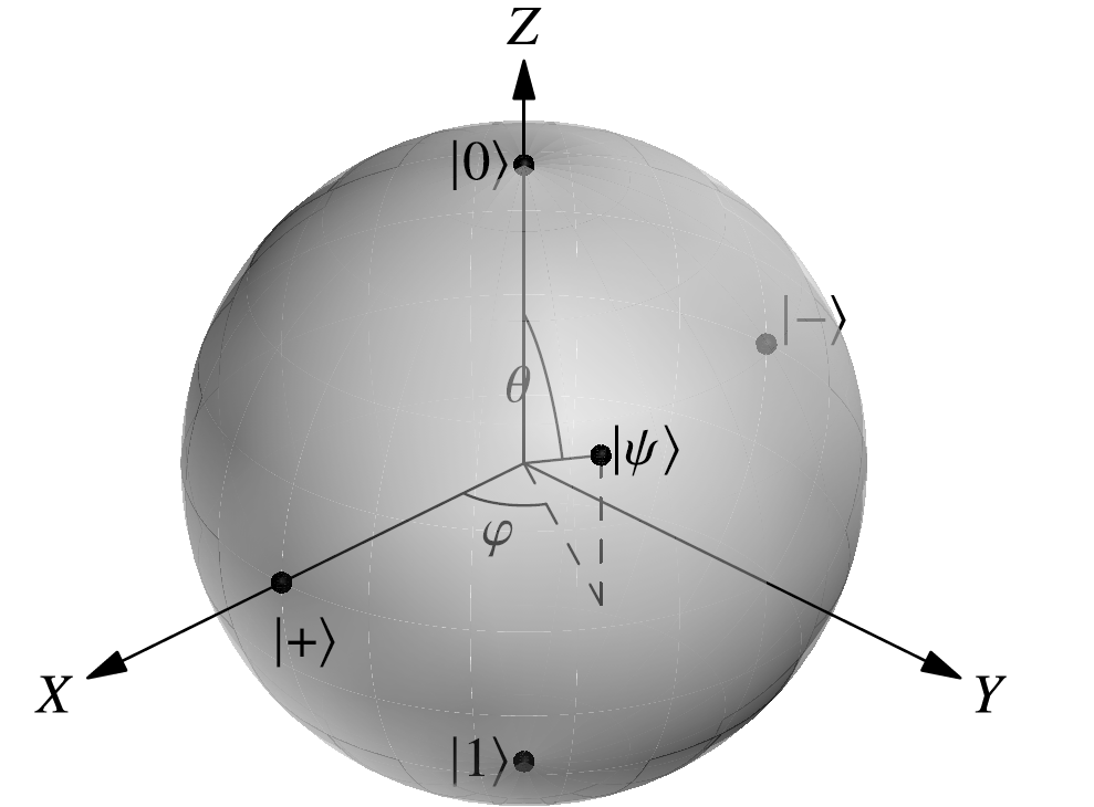
In this way, we can describe the state of any qubit with just two numbers $\theta \in \left\lbrack {0,\pi} \right\rbrack$ and $\varphi \in \left\lbrack {0,2\pi} \right\rbrack$ that we can interpret as a polar angle and an azimuthal angle, respectively (that is, we are using what are known as spherical coordinates). This gives us a three-dimensional point

$(\sin\theta\cos\varphi,\sin\theta\sin\varphi,\cos\theta)$

that locates the state of the qubit on the surface of a sphere, called the Bloch sphere (see Figure 1.2).

Figure 1.2: Qubit state \left| \psi \right\rangle represented on the Bloch sphere. — **Figure 1.2**: Qubit state $\left| \psi \right\rangle$ represented on the Bloch sphere.

**Figure 1.2**: Qubit state $\left| \psi \right\rangle$ represented on the Bloch sphere.

Notice that $\theta$ runs from to $\pi$ to cover the whole range from the top to the bottom of the sphere. This is why we used $\left. \theta\slash 2 \right.$ in the representation of our preceding qubit. We only needed to get up to $\left. \pi\slash 2 \right.$ for our angles in the sines and cosines!

In the Bloch sphere, $\left| 0 \right\rangle$ is mapped to the North pole and $\left| 1 \right\rangle$ to the South pole. In general, states that are orthogonal with respect to the inner product are antipodal on the sphere. For instance, $\left| + \right\rangle$ and $\left| - \right\rangle$ both lie on the equator, but on opposite points of the sphere. As we already know, the gate takes $\left| 0 \right\rangle$ to $\left| 1 \right\rangle$ and $\left| 1 \right\rangle$ to $\left| 0 \right\rangle$ , but leaves $\left| + \right\rangle$ and $\left| - \right\rangle$ unchanged, at least up to an irrelevant global phase. In fact, this means that the gate acts like a rotation of $\pi$ radians around the axis of the Bloch sphere…, so now you know why we use that name for the gate! In the same manner, and are rotations of $\pi$ radians around the and axes, respectively.

We can generalize this behavior to obtain rotations of any angle around any axis of the Bloch sphere. For instance, for the , , and axes we may define

$R_{X}(\theta) = e^{- i\frac{\theta}{2}X} = \cos\frac{\theta}{2}I - i\sin\frac{\theta}{2}X = \begin{pmatrix} {\cos\frac{\theta}{2}} & {- i\sin\frac{\theta}{2}} \\ {- i\sin\frac{\theta}{2}} & {\cos\frac{\theta}{2}} \\ \end{pmatrix},$

$R_{Y}(\theta) = e^{- i\frac{\theta}{2}Y} = \cos\frac{\theta}{2}I - i\sin\frac{\theta}{2}Y = \begin{pmatrix} {\cos\frac{\theta}{2}} & {- \sin\frac{\theta}{2}} \\ {\sin\frac{\theta}{2}} & {\cos\frac{\theta}{2}} \\ \end{pmatrix},$

$R_{Z}(\theta) = e^{- i\frac{\theta}{2}Z} = \cos\frac{\theta}{2}I - i\sin\frac{\theta}{2}Z = \begin{pmatrix} e^{- i\frac{\theta}{2}} & 0 \\ 0 & e^{i\frac{\theta}{2}} \\ \end{pmatrix} \equiv \begin{pmatrix} 1 & 0 \\ 0 & e^{i\theta} \\ \end{pmatrix},$

where we use the $\equiv$ symbol for equivalent action up to a global phase. Notice that $R_{X}(\pi) \equiv X$ , $R_{Y}(\pi) \equiv Y$ , $R_{Z}(\pi) \equiv Z$ , $R_{Z}(\frac{\pi}{2}) \equiv S$ , and $R_{Z}(\frac{\pi}{4}) \equiv T$ .

Exercise 1.7

Check these equivalences by substituting the angles in the definitions of $R_{X}$ , $R_{Y}$ , and $R_{Z}$ .

In fact, it can be proved (see, for instance, the book by Nielsen and Chuang [69]) that for any one-qubit gate there exists a unit vector $r = (r_{x},r_{y},r_{z})$ and an angle $\theta$ such that

$U \equiv \cos\frac{\theta}{2}I - i\sin\frac{\theta}{2}(r_{x}X + r_{y}Y + r_{z}Z).$

For example, choosing $\theta = \pi$ and $\left. r = (1\slash\sqrt{2},0,1\slash\sqrt{2}) \right.$ we can obtain the Hadamard gate, for it holds that

$H \equiv - i\frac{1}{\sqrt{2}}(X + Z).$

Additionally, it can also be proved that, again for any one-qubit gate , there exist three angles $\alpha$ , $\beta$ , and $\gamma$ such that

$U \equiv R_{Z}(\alpha)R_{Y}(\beta)R_{Z}(\gamma).$

In fact, you can obtain such a decomposition for any two rotation axes as long as they are not parallel, not just for and .

Moreover, in some quantum computing architectures (including the ones used by companies such as IBM), it is common to use a universal one-qubit gate, called the -gate, that depends on three angles and is able to generate any other one-qubit gate. Its matrix is

$U\left( {\theta,\varphi,\lambda} \right) = \begin{pmatrix} {\cos\frac{\theta}{2}} & {- e^{i\lambda}\sin\frac{\theta}{2}} \\ {e^{i\varphi}\sin\frac{\theta}{2}} & {e^{i{({\varphi + \lambda})}}\cos\frac{\theta}{2}} \\ \end{pmatrix}.$

Exercise 1.8

Show that $U\left( {\theta,\varphi,\lambda} \right)$ is unitary. Check that $\left. R_{X}(\theta) = U(\theta, - \pi\slash 2,\pi\slash 2) \right.$ , that $R_{Y}(\theta) = U(\theta,0,0)$ and that, up to a global phase, $U(\theta) = R_{Z}(0,0,\theta)$ .

All these observations about how to construct one-qubit gates from rotations and parametrized families will be very important when we talk about variational forms and feature maps in Chapter 9, Quantum Support Vector Machines, and Chapter 10, Quantum Neural Networks, and also to construct controlled gates later in this chapter.

1.3.5 Hello, quantum world!

To put together everything that we have learned, we are going to create our very first complete quantum circuit. It looks like this:

It doesn't seem very impressive, but let's analyze it part by part. As you know, following convention, the initial state of our qubit is assumed to be $\left| 0 \right\rangle$ , so that's what we have before we do anything. Then we apply the gate, so the state changes to $\sqrt{\left. 1\slash 2 \right.}\left| 0 \right\rangle + \sqrt{\left. 1\slash 2 \right.}\left| 1 \right\rangle$ . Finally, we measure the qubit. The probability of obtaining will be $\left. \left| \sqrt{\left. 1\slash 2 \right.} \right|^{2} = 1\slash 2 \right.$ , and that of getting will also be $\left. 1\slash 2 \right.$ , so we have created a circuit that — at least in theory — generates random bits following a perfectly uniform distribution.

To learn more…

Unbiased uniform bit distributions are of great relevance for multiple applications in simulation, cryptography, and even online gambling games. As we will learn in Chapter 2, The Tools of the Trade, current quantum computers deviate from this equilibrium because they are affected by noise and gate and measurement errors. However, protocols to extract perfect random bits even with noisy quantum computers have been proposed and could become one of the first practical applications of quantum computing (see, for instance, the paper by Acín and Masanes [3]).

We can modify the previous circuit to obtain any distribution over and that we desire. If we want the probability of measuring to be $p \in \left\lbrack {0,1} \right\rbrack$ , we just need to consider $\theta = 2\arccos\sqrt{p}$ and the following circuit:

R (𝜃) Y

Exercise 1.9

Check that, with the preceding circuit, the state before measurement is $\sqrt{p}\left| 0 \right\rangle + \sqrt{1 - p}\left| 1 \right\rangle$ and, hence, the probability of measuring is and that of measuring is 1 - p .

For now, this is all that we need to know about one-qubit states, gates, and measurements. Let us move on to two-qubit systems, where the mysteries of entanglement are awaiting to be revealed!

You have been reading a chapter from

A Practical Guide to Quantum Machine Learning and Quantum Optimization

Published in: Mar 2023Publisher: PacktISBN-13: 9781804613832

A free Packt account unlocks extra newsletters, articles, discounted offers, and much more. Start advancing your knowledge today.

undefined

Unlock this book and the full library FREE for 7 days

Get unlimited access to 7000+ expert-authored eBooks and videos courses covering every tech area you can think of

Start free trial

Renews at $15.99/month. Cancel anytime

Authors (2)

Elías F. Combarro

Elías F. Combarro holds degrees from the University of Oviedo (Spain) in both Mathematics (1997, award for second highest grades in the country) and Computer Science (2002, award for highest grades in the country). After some research stays at the Novosibirsk State University (Russia), he obtained a Ph.D. in Mathematics (Oviedo, 2001) with a dissertation on the properties of some computable predicates under the supervision of Prof. Andrey Morozov and Prof. Consuelo Martínez. Since 2009, Elías F. Combarro has been an associate professor at the Computer Science Department of the University of Oviedo. He has published more than 50 research papers in international journals on topics such as Computability Theory, Machine Learning, Fuzzy Measures and Computational Algebra. His current research focuses on the application Quantum Computing to algebraic, optimisation and machine learning problems. From July 2020 to January 2021, he was a Cooperation Associate at CERN openlab. Currently, he is the Spain representative in the Advisory Board of CERN Quantum Technology Initiative, a member of the Advisory Board of SheQuantum and one of the founders of the QSpain, a quantum computing think tank based in Spain.
Read more about Elías F. Combarro

Samuel González-Castillo

Samuel González-Castillo holds degrees from the University of Oviedo (Spain) in both Mathematics and Physics (2021). He is currently a mathematics research student at the National University of Ireland, Maynooth, where he works as a graduate teaching assistant. He completed his physics bachelor thesis under the supervision of Prof. Elías F. Combarro and Prof. Ignacio F. Rúa (University of Oviedo), and Dr. Sofia Vallecorsa (CERN). In it, he worked alongside other researchers from ETH Zürich on the application of Quantum Machine Learning to classification problems in High Energy Physis. In 2021, he was a summer student at CERN developing a benchmarking framework for quantum simulators. He has contributed to several conferences on quantum computing.
Read more about Samuel González-Castillo

Personalised recommendations for you

Based on your interests and search pattern

C++ Programming for Linux Systems

This book covers the essential system programming tools and helps you explore the features of C++20. It emphasizes important details to maintain code quality and tackle everyday challenges of developing software for high performance, optimization, and more.

BookSep 2023288 pages

Expert C++

Discover advanced programming techniques, the latest features of C++17 and C++20, and best practices for memory management, debugging, testing, and large-scale application design with Expert C++. Ideal for experienced developers advancing to proficient programmers and building professional-grade C++ applications.

BookAug 2023604 pages

iOS 17 Programming for Beginners

iOS 17 Programming for Beginners, Eighth Edition is your comprehensive guide to learning the art of iOS app development. Whether you dream of creating the next chart-topping app or simply want to enhance your programming skills, this book is your trusted companion on this exciting journey.

BookOct 2023604 pages4

Developer Career Masterplan

Written by industry experts that have spent the last 20+ years helping developers grow their career path towards senior developer positions and beyond. This book provides a comprehensive guide, sharing examples and stories from their global careers. By the end, you’ll have the knowledge to create a clear career progression plan as a technical professional.

BookSep 2023310 pages

Refactoring with C#

In Refactoring with C#, you’ll explore the process of safely refactoring modern .NET code using Visual Studio features, advanced unit tests, AI assistance, and custom Roslyn analyzers.

BookNov 2023434 pages

Python Real-World Projects

Amplify your developer journey by curating a dynamic project portfolio that outshines traditional resumes. Delve into the Python realm through immersive projects, mastering core concepts while constructing comprehensive modules and applications. From data acquisition prowess to impactful data visualization, Python Real-World Projects arms you with essential skills to beat the competition.

BookSep 2023478 pages5

The MVVM Pattern in .NET MAUI

The MVVM Pattern in .NET MAUI enables developers to master MVVM principles and effectively apply them to .NET MAUI. This book uses real-life examples and covers complex problems to help you successfully apply MVVM with .NET MAUI to confidently develop robust and high-performing cross-platform apps.

BookNov 2023386 pages

Extending Microsoft Business Central with Power Platform

Extending Business Central with the Power Platform is a step-by-step guide for Business Central professionals to create solutions that automate business processes, explain complex workflow approvals, and integrate with hundreds of other systems, without traditional development. It’ll guide you in customizing Business Central with Power Platform.

BookAug 2023458 pages5

Extending Microsoft Business Central with Power Platform

Extending Business Central with the Power Platform is a step-by-step guide for Business Central professionals to create solutions that automate business processes, explain complex workflow approvals, and integrate with hundreds of other systems, without traditional development. It’ll guide you in customizing Business Central with Power Platform.

BookAug 2023458 pages5

Quantum Computing Algorithms

The book emphasizes intuitive ideas behind quantum algorithms in ways that other books don’t cover, striking a careful balance between no math and too much math. To get the most from this book, you should be comfortable with basic algebra and writing simple computer code. No prior understanding of quantum physics is needed to get started.

BookSep 2023342 pages

Python – Complete Python, Django, Data Science and ML Guide

Unlock Python's full potential with this 50+ hour course! From programming to web and game development, data manipulation, and machine learning, gain the skills required to succeed in various Python-related careers. With practical tasks, hands-on experience, and a strong foundation in Python, you'll be ready to tackle real-world challenges and take advantage of the many opportunities this versatile language offers.

VideoNov 202350 hours 30 minutes5

Python – Complete Python, Django, Data Science and ML Guide

Unlock Python's full potential with this 50+ hour course! From programming to web and game development, data manipulation, and machine learning, gain the skills required to succeed in various Python-related careers. With practical tasks, hands-on experience, and a strong foundation in Python, you'll be ready to tackle real-world challenges and take advantage of the many opportunities this versatile language offers.

VideoNov 202350 hours 30 minutes5