


In both classical and Bayesian approaches, a probability distribution function is the central quantity, which captures all of the information about the relationship between variables in the presence of uncertainty. A probability distribution assigns a probability value to each measurable subset of outcomes of a random experiment. The variable involved could be discrete or continuous, and univariate or multivariate. Although people use slightly different terminologies, the commonly used probability distributions for the different types of random variables are as follows:
One of the well-known distribution functions is the normal or Gaussian distribution, which is named after Carl Friedrich Gauss, a famous German mathematician and physicist. It is also known by the name bell curve because of its shape. The mathematical form of this distribution is given by:
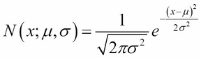
Here,  is the mean or location parameter and
  is the standard deviation or scale parameter (
 is called variance). The following graphs show what the distribution looks like for different values of location and scale parameters:
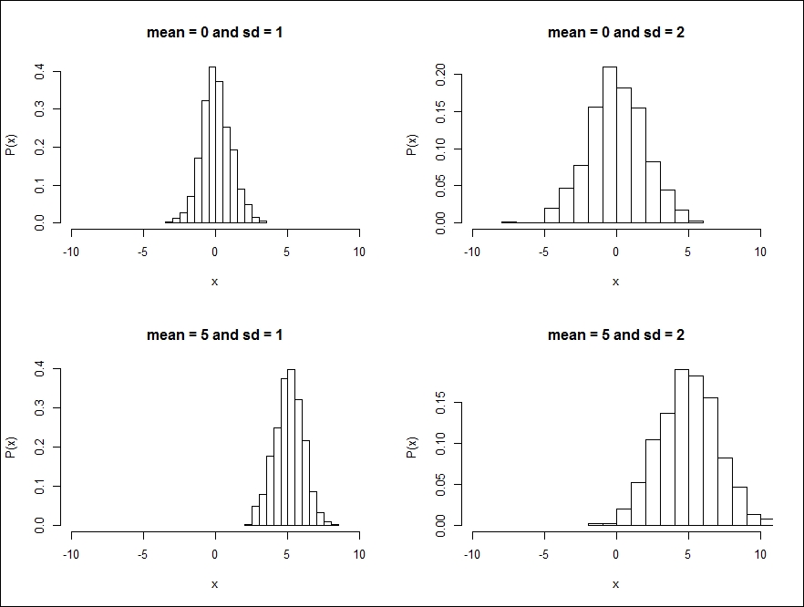
One can see that as the mean changes, the location of the peak of the distribution changes. Similarly, when the standard deviation changes, the width of the distribution also changes.
Many natural datasets follow normal distribution because, according to the central limit theorem, any random variable that can be composed as a mean of independent random variables will have a normal distribution. This is irrespective of the form of the distribution of this random variable, as long as they have finite mean and variance and all are drawn from the same original distribution. A normal distribution is also very popular among data scientists because in many statistical inferences, theoretical results can be derived if the underlying distribution is normal.
Now, let us look at the multidimensional version of normal distribution. If the random variable is an N-dimensional vector, x is denoted by:
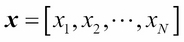
Then, the corresponding normal distribution is given by:
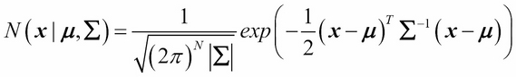
Here,  corresponds to the mean (also called location) and
  is an N x N covariance matrix (also called scale).
To get a better understanding of the multidimensional normal distribution, let us take the case of two dimensions. In this case,  and the covariance matrix is given by:
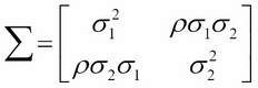
Here,  and
and  are the variances along
  and
and  directions, and
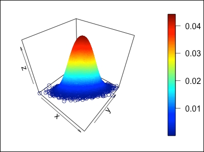
  is the correlation between and . A plot of two-dimensional normal distribution for
  ,
,  , and
, and  is shown in the following image:
If  , then the two-dimensional normal distribution will be reduced to the product of two one-dimensional normal distributions, since would become diagonal in this case. The following 2D projections of normal distribution for the same values of and but with and
  illustrate this case:
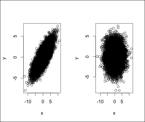
The high correlation between x and y in the first case forces most of the data points along the 45 degree line and makes the distribution more anisotropic; whereas, in the second case, when the correlation is zero, the distribution is more isotropic.
We will briefly review some of the other well-known distributions used in Bayesian inference here.


