Predicting Continuous Target Variables with Regression Analysis

Throughout the previous chapters, you learned a lot about the main concepts behind supervised learning and trained many different models for classification tasks to predict group memberships or categorical variables. In this chapter, we will dive into another subcategory of supervised learning: regression analysis.

Regression models are used to predict target variables on a continuous scale, which makes them attractive for addressing many questions in science. They also have applications in industry, such as understanding relationships between variables, evaluating trends, or making forecasts. One example is predicting the sales of a company in future months.

In this chapter, we will discuss the main concepts of regression models and cover the following topics:

• Exploring and visualizing datasets
• Looking at different approaches to implement linear regression models
• Training regression models that...

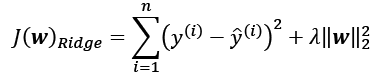
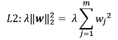
Introducing linear regression

The goal of linear regression is to model the relationship between one or multiple features and a continuous target variable. In contrast to classification—a different subcategory of supervised learning—regression analysis aims to predict outputs on a continuous scale rather than categorical class labels.

In the following subsections, you will be introduced to the most basic type of linear regression, simple linear regression, and understand how to relate it to the more general, multivariate case (linear regression with multiple features).

Simple linear regression

The goal of simple (univariate) linear regression is to model the relationship between a single feature (explanatory variable, x) and a continuous-valued target (response variable, y). The equation of a linear model with one explanatory variable is defined as follows:

Here, the weight, , represents the y axis intercept and is the weight coefficient of the explanatory...

Exploring the Housing dataset

Before we implement the first linear regression model, we will discuss a new dataset, the Housing dataset, which contains information about houses in the suburbs of Boston collected by D. Harrison and D.L. Rubinfeld in 1978. The Housing dataset has been made freely available and is included in the code bundle of this book. The dataset has recently been removed from the UCI Machine Learning Repository but is available online at https://raw.githubusercontent.com/rasbt/python-machine-learning-book-3rd-edition/master/ch10/housing.data.txt or scikit-learn (https://github.com/scikit-learn/scikit-learn/blob/master/sklearn/datasets/data/boston_house_prices.csv). As with each new dataset, it is always helpful to explore the data through a simple visualization, to get a better feeling of what we are working with.

Loading the Housing dataset into a data frame

In this section, we will load the Housing dataset using the pandas read_csv function, which is fast...

Implementing an ordinary least squares linear regression model

At the beginning of this chapter, it was mentioned that linear regression can be understood as obtaining the best-fitting straight line through the examples of our training data. However, we have neither defined the term best-fitting nor have we discussed the different techniques of fitting such a model. In the following subsections, we will fill in the missing pieces of this puzzle using the ordinary least squares (OLS) method (sometimes also called linear least squares) to estimate the parameters of the linear regression line that minimizes the sum of the squared vertical distances (residuals or errors) to the training examples.

Solving regression for regression parameters with gradient descent

Consider our implementation of the Adaptive Linear Neuron (Adaline) from Chapter 2, Training Simple Machine Learning Algorithms for Classification. You will remember that the artificial neuron uses a linear activation function...

Fitting a robust regression model using RANSAC

Linear regression models can be heavily impacted by the presence of outliers. In certain situations, a very small subset of our data can have a big effect on the estimated model coefficients. There are many statistical tests that can be used to detect outliers, which are beyond the scope of the book. However, removing outliers always requires our own judgment as data scientists as well as our domain knowledge.

As an alternative to throwing out outliers, we will look at a robust method of regression using the RANdom SAmple Consensus (RANSAC) algorithm, which fits a regression model to a subset of the data, the so-called inliers.

We can summarize the iterative RANSAC algorithm as follows:

1. Select a random number of examples to be inliers and fit the model.
2. Test all other data points against the fitted model and add those points that fall within a user-given tolerance to the inliers.
3. Refit the model using all inliers...

Evaluating the performance of linear regression models

In the previous section, you learned how to fit a regression model on training data. However, you discovered in previous chapters that it is crucial to test the model on data that it hasn't seen during training to obtain a more unbiased estimate of its generalization performance.

As you will remember from Chapter 6, Learning Best Practices for Model Evaluation and Hyperparameter Tuning, we want to split our dataset into separate training and test datasets, where we will use the former to fit the model and the latter to evaluate its performance on unseen data to estimate the generalization performance. Instead of proceeding with the simple regression model, we will now use all variables in the dataset and train a multiple regression model:

>>> from sklearn.model_selection import train_test_split
>>> X = df.iloc[:, :-1].values
>>> y = df['MEDV'].values
>>> X_train, X_test,...

Using regularized methods for regression

As we discussed in Chapter 3, A Tour of Machine Learning Classifiers Using scikit-learn, regularization is one approach to tackling the problem of overfitting by adding additional information, and thereby shrinking the parameter values of the model to induce a penalty against complexity. The most popular approaches to regularized linear regression are the so-called Ridge Regression, least absolute shrinkage and selection operator (LASSO), and elastic Net.

Ridge Regression is an L2 penalized model where we simply add the squared sum of the weights to our least-squares cost function:

Here:

By increasing the value of hyperparameter , we increase the regularization strength and thereby shrink the weights of our model. Please note that we don't regularize the intercept term, .

An alternative approach that can lead to sparse models is LASSO. Depending on the regularization strength, certain weights can become zero, which also...

Turning a linear regression model into a curve – polynomial regression

In the previous sections, we assumed a linear relationship between explanatory and response variables. One way to account for the violation of linearity assumption is to use a polynomial regression model by adding polynomial terms:

Here, d denotes the degree of the polynomial. Although we can use polynomial regression to model a nonlinear relationship, it is still considered a multiple linear regression model because of the linear regression coefficients, w. In the following subsections, we will see how we can add such polynomial terms to an existing dataset conveniently and fit a polynomial regression model.

Adding polynomial terms using scikit-learn

We will now learn how to use the PolynomialFeatures transformer class from scikit-learn to add a quadratic term (d = 2) to a simple regression problem with one explanatory variable. Then, we will compare the polynomial to the linear fit by following...

Dealing with nonlinear relationships using random forests

In this section, we are going to take a look at random forest regression, which is conceptually different from the previous regression models in this chapter. A random forest, which is an ensemble of multiple decision trees, can be understood as the sum of piecewise linear functions, in contrast to the global linear and polynomial regression models that we discussed previously. In other words, via the decision tree algorithm, we subdivide the input space into smaller regions that become more manageable.

Decision tree regression

An advantage of the decision tree algorithm is that it does not require any transformation of the features if we are dealing with nonlinear data, because decision trees analyze one feature at a time, rather than taking weighted combinations into account. (Likewise, normalizing or standardizing features is not required for decision trees.) You will remember from Chapter 3, A Tour of Machine Learning...

Summary

At the beginning of this chapter, you learned about simple linear regression analysis to model the relationship between a single explanatory variable and a continuous response variable. We then discussed a useful explanatory data analysis technique to look at patterns and anomalies in data, which is an important first step in predictive modeling tasks.

We built our first model by implementing linear regression using a gradient-based optimization approach. You then saw how to utilize scikit-learn's linear models for regression and also implement a robust regression technique (RANSAC) as an approach for dealing with outliers. To assess the predictive performance of regression models, we computed the mean sum of squared errors and the related metric. Furthermore, we also discussed a useful graphical approach to diagnose the problems of regression models: the residual plot.

After we explored how regularization can be applied to regression models to reduce the model...