


Classification tasks and decision boundaries
Till now, the focus of the chapter was on regression. In this section, we will talk about another important task: the task of classification. Let us first understand the difference between regression (also sometimes referred to as prediction) and classification:
- In classification, the data is grouped into classes/categories, while in regression, the aim is to get a continuous numerical value for given data. For example, identifying the number of handwritten digits is a classification task; all handwritten digits will belong to one of the ten numbers lying between 0-9. The task of predicting the price of the house depending upon different input variables is a regression task.
- In a classification task, the model finds the decision boundaries separating one class from another. In the regression task, the model approximates a function that fits the input-output relationship.
- Classification is a subset of regression; here, we are predicting classes. Regression is much more general.
Figure 2.8 shows how classification and regression tasks differ. In classification, we need to find a line (or a plane or hyperplane in multidimensional space) separating the classes. In regression, the aim is to find a line (or plane or hyperplane) that fits the given input points:
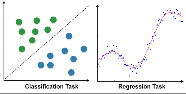
Figure 2.8: Classification vs regression
In the following section, we will explain logistic regression, which is a very common and useful classification technique.
Logistic regression
Logistic regression is used to determine the probability of an event. Conventionally, the event is represented as a categorical dependent variable. The probability of the event is expressed using the sigmoid (or “logit”) function:

The goal now is to estimate weights  and bias term b. In logistic regression, the coefficients are estimated using either the maximum likelihood estimator or stochastic gradient descent. If p is the total number of input data points, the loss is conventionally defined as a cross-entropy term given by:

Logistic regression is used in classification problems. For example, when looking at medical data, we can use logistic regression to classify whether a person has cancer or not. If the output categorical variable has two or more levels, we can use multinomial logistic regression. Another common technique used for two or more output variables is one versus all.
For multiclass logistic regression, the cross-entropy loss function is modified as:

where K is the total number of classes. You can read more about logistic regression at https://en.wikipedia.org/wiki/Logistic_regression.
Now that you have some idea about logistic regression, let us see how we can apply it to any dataset.
Logistic regression on the MNIST dataset
Next, we will use TensorFlow Keras to classify handwritten digits using logistic regression. We will be using the MNIST (Modified National Institute of Standards and Technology) dataset. For those working in the field of deep learning, MNIST is not new, it is like the ABC of machine learning. It contains images of handwritten digits and a label for each image, indicating which digit it is. The label contains a value lying between 0-9 depending on the handwritten digit. Thus, it is a multiclass classification.
To implement the logistic regression, we will make a model with only one dense layer. Each class will be represented by a unit in the output, so since we have 10 classes, the number of units in the output would be 10. The probability function used in the logistic regression is similar to the sigmoid activation function; therefore, we use sigmoid activation.
Let us build our model:
- The first step is, as always, importing the modules needed. Notice that here we are using another useful layer from the Keras API, the
Flattenlayer. TheFlattenlayer helps us to resize the 28 x 28 two-dimensional input images of the MNIST dataset into a 784 flattened array:import tensorflow as tf import numpy as np import matplotlib.pyplot as plt import pandas as pd import tensorflow.keras as K from tensorflow.keras.layers import Dense, Flatten - We take the input data of MNIST from the
tensorflow.kerasdataset:((train_data, train_labels),(test_data, test_labels)) = tf.keras.datasets.mnist.load_data() - Next, we preprocess the data. We normalize the images; the MNIST dataset images are black and white images with the intensity value of each pixel lying between 0-255. We divide it by 255, so that now the values lie between 0-1:
train_data = train_data/np.float32(255) train_labels = train_labels.astype(np.int32) test_data = test_data/np.float32(255) test_labels = test_labels.astype(np.int32) - Now, we define a very simple model; it has only one
Denselayer with10units, and it takes an input of size 784. You can see from the output of the model summary that only theDenselayer has trainable parameters:model = K.Sequential([ Flatten(input_shape=(28, 28)), Dense(10, activation='sigmoid') ]) model.summary()Model: "sequential" ____________________________________________________________ Layer (type) Output Shape Param # ============================================================ flatten (Flatten) (None, 784) 0 dense (Dense) (None, 10) 7850 ============================================================ Total params: 7,850 Trainable params: 7,850 Non-trainable params: 0 ____________________________________________________________ - Since the test labels are integral values, we will use
SparseCategoricalCrossentropyloss withlogitsset toTrue. The optimizer selected is Adam. Additionally, we also define accuracy as metrics to be logged as the model is trained. We train our model for 50 epochs, with a train-validation split of 80:20:model.compile(optimizer='adam', loss=tf.keras.losses.SparseCategoricalCrossentropy(from_logits=True), metrics=['accuracy']) history = model.fit(x=train_data,y=train_labels, epochs=50, verbose=1, validation_split=0.2) - Let us see how our simple model has fared by plotting the loss plot. You can see that since the validation loss and training loss are diverging, as the training loss is decreasing, the validation loss increases, thus the model is overfitting. You can improve the model performance by adding hidden layers:
plt.plot(history.history['loss'], label='loss')
plt.plot(history.history['val_loss'], label='val_loss')
plt.xlabel('Epoch')
plt.ylabel('Loss')
plt.legend()
plt.grid(True)
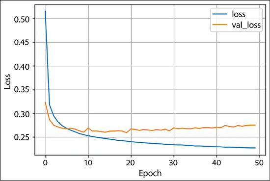
Figure 2.9: Loss plot
- To better understand the result, we build two utility functions; these functions help us in visualizing the handwritten digits and the probability of the 10 units in the output:
def plot_image(i, predictions_array, true_label, img): true_label, img = true_label[i], img[i] plt.grid(False) plt.xticks([]) plt.yticks([]) plt.imshow(img, cmap=plt.cm.binary) predicted_label = np.argmax(predictions_array) if predicted_label == true_label: color ='blue' else: color ='red' plt.xlabel("Pred {} Conf: {:2.0f}% True ({})".format(predicted_label, 100*np.max(predictions_array), true_label), color=color) def plot_value_array(i, predictions_array, true_label): true_label = true_label[i] plt.grid(False) plt.xticks(range(10)) plt.yticks([]) thisplot = plt.bar(range(10), predictions_array, color"#777777") plt.ylim([0, 1]) predicted_label = np.argmax(predictions_array) thisplot[predicted_label].set_color('red') thisplot[true_label].set_color('blue') - Using these utility functions, we plot the predictions:
predictions = model.predict(test_data) i = 56 plt.figure(figsize=(10,5)) plt.subplot(1,2,1) plot_image(i, predictions[i], test_labels, test_data) plt.subplot(1,2,2) plot_value_array(i, predictions[i], test_labels) plt.show() - The plot on the left is the image of the handwritten digit, with the predicted label, the confidence in the prediction, and the true label. The image on the right shows the probability (logistic) output of the 10 units; we can see that the unit which represents the number 4 has the highest probability:
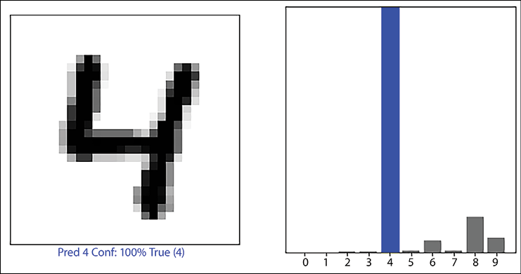
Figure 2.10: Predicted digit and confidence value of the prediction
- In this code, to stay true to logistic regression, we used a sigmoid activation function and only one
Denselayer. For better performance, adding dense layers and using softmax as the final activation function will be helpful. For example, the following model gives 97% accuracy on the validation dataset:better_model = K.Sequential([ Flatten(input_shape=(28, 28)), Dense(128, activation='relu'), Dense(10, activation='softmax') ]) better_model.summary()
You can experiment by adding more layers, or by changing the number of neurons in each layer, and even changing the optimizer. This will give you a better understanding of how these parameters influence the model performance.