

A roadmap for building machine learning systems
In previous sections, we discussed the basic concepts of machine learning and the three different types of learning. In this section, we will discuss the other important parts of a machine learning system accompanying the learning algorithm.
The following diagram shows a typical workflow for using machine learning in predictive modeling, which we will discuss in the following subsections:
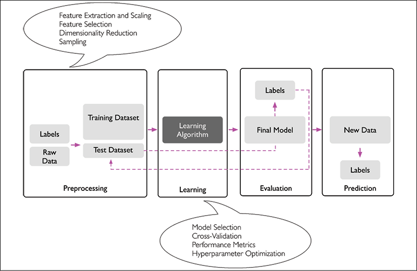
Preprocessing – getting data into shape
Let's begin with discussing the roadmap for building machine learning systems. Raw data rarely comes in the form and shape that is necessary for the optimal performance of a learning algorithm. Thus, the preprocessing of the data is one of the most crucial steps in any machine learning application.
If we take the Iris flower dataset from the previous section as an example, we can think of the raw data as a series of flower images from which we want to extract meaningful features. Useful features could be the color, hue, and intensity of the flowers, or the height, length, and width of the flowers.
Many machine learning algorithms also require that the selected features are on the same scale for optimal performance, which is often achieved by transforming the features in the range [0, 1] or a standard normal distribution with zero mean and unit variance, as we will see in later chapters.
Some of the selected features may be highly correlated and therefore redundant to a certain degree. In those cases, dimensionality reduction techniques are useful for compressing the features onto a lower dimensional subspace. Reducing the dimensionality of our feature space has the advantage that less storage space is required, and the learning algorithm can run much faster. In certain cases, dimensionality reduction can also improve the predictive performance of a model if the dataset contains a large number of irrelevant features (or noise); that is, if the dataset has a low signal-to-noise ratio.
To determine whether our machine learning algorithm not only performs well on the training dataset but also generalizes well to new data, we also want to randomly divide the dataset into a separate training and test dataset. We use the training dataset to train and optimize our machine learning model, while we keep the test dataset until the very end to evaluate the final model.
Training and selecting a predictive model
As you will see in later chapters, many different machine learning algorithms have been developed to solve different problem tasks. An important point that can be summarized from David Wolpert's famous No free lunch theorems is that we can't get learning "for free" (The Lack of A Priori Distinctions Between Learning Algorithms, D.H. Wolpert, 1996; No free lunch theorems for optimization, D.H. Wolpert and W.G. Macready, 1997). We can relate this concept to the popular saying, "I suppose it is tempting, if the only tool you have is a hammer, to treat everything as if it were a nail" (Abraham Maslow, 1966). For example, each classification algorithm has its inherent biases, and no single classification model enjoys superiority if we don't make any assumptions about the task. In practice, it is therefore essential to compare at least a handful of different algorithms in order to train and select the best performing model. But before we can compare different models, we first have to decide upon a metric to measure performance. One commonly used metric is classification accuracy, which is defined as the proportion of correctly classified instances.
One legitimate question to ask is this: how do we know which model performs well on the final test dataset and real-world data if we don't use this test dataset for the model selection, but keep it for the final model evaluation? In order to address the issue embedded in this question, different techniques summarized as "cross-validation" can be used. In cross-validation, we further divide a dataset into training and validation subsets in order to estimate the generalization performance of the model. Finally, we also cannot expect that the default parameters of the different learning algorithms provided by software libraries are optimal for our specific problem task. Therefore, we will make frequent use of hyperparameter optimization techniques that help us to fine-tune the performance of our model in later chapters.
We can think of those hyperparameters as parameters that are not learned from the data but represent the knobs of a model that we can turn to improve its performance. This will become much clearer in later chapters when we see actual examples.
Evaluating models and predicting unseen data instances
After we have selected a model that has been fitted on the training dataset, we can use the test dataset to estimate how well it performs on this unseen data to estimate the so-called generalization error. If we are satisfied with its performance, we can now use this model to predict new, future data. It is important to note that the parameters for the previously mentioned procedures, such as feature scaling and dimensionality reduction, are solely obtained from the training dataset, and the same parameters are later reapplied to transform the test dataset, as well as any new data instances—the performance measured on the test data may be overly optimistic otherwise.