Reader small image

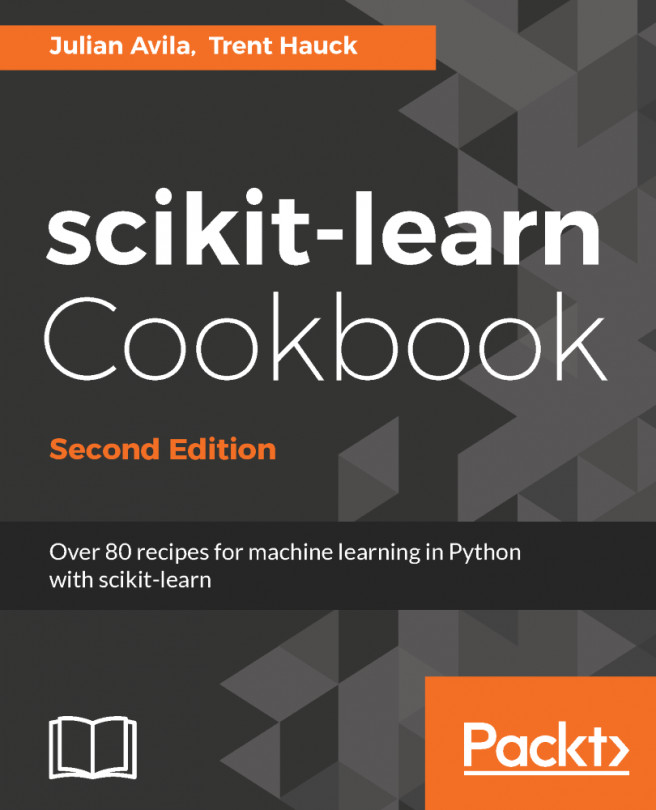
You're reading from  scikit-learn Cookbook - Second Edition

Product typeBook
Published inNov 2017
Reading LevelIntermediate
PublisherPackt
ISBN-139781787286382
Edition2nd Edition
Languages
Right arrow
Author (1)
Trent Hauck
Trent Hauck
author image
Trent Hauck

Trent Hauck is a data scientist living and working in the Seattle area. He grew up in Wichita, Kansas and received his undergraduate and graduate degrees from the University of Kansas. He is the author of the book Instant Data Intensive Apps with pandas How-to, Packt Publishing—a book that can get you up to speed quickly with pandas and other associated technologies.
Read more about Trent Hauck

Right arrow

Cross-Validation and Post-Model Workflow

In this chapter, we will cover the following recipes:

  • Selecting a model with cross-validation
  • K-fold cross-validation
  • Balanced cross-validation
  • Cross-validation with ShuffleSplit
  • Time series cross-validation
  • Grid search with scikit-learn
  • Randomized search with scikit-learn
  • Classification metrics
  • Regression metrics
  • Clustering metrics
  • Using dummy estimators to compare results
  • Feature selection
  • Feature selection on L1 norms
  • Persisting models with joblib or pickle
Introduction

This is perhaps the most important chapter. The fundamental question addressed in this chapter is as follows:

  • How do we select a model that predicts well?

This is the purpose of cross-validation, regardless of what the model is. This is slightly different from traditional statistics, which is perhaps more concerned with how we understand a phenomenon better. (Why would I limit my quest for understanding? Well, because there is more and more data, we cannot necessarily look at it all, reflect upon it, and create a theoretical model.)

Machine learning is concerned with prediction and how a machine learning algorithm processes new unseen data and arrives at predictions. Even if it does not seem like traditional statistics, you can use interpretation and domain understanding to create new columns (features) and make even better predictions. You can use traditional statistics...

Selecting a model with cross-validation

We saw automatic cross-validation, the cross_val_score function, in Chapter 1, High-Performance Machine Learning – NumPy. This will be very similar, except we will use the last two columns of the iris dataset as the data. The purpose of this section is to select the best model we can.

Before starting, we will define the best model as the one that scores the highest. If there happens to be a tie, we will choose the model that has the best score with the least volatility.

Getting ready

In this recipe we will do the following:

  • Load the last two features (columns) of the iris dataset
  • Split the data into training and testing data
  • Instantiate two k-nearest neighbors (KNN) algorithms...

K-fold cross validation

In the quest to find the best model, you can view the indices of cross-validation folds and see what data is in each fold.

Getting ready

Create a toy dataset that is very small:

import numpy as np
X = np.array([[1, 2], [3, 4], [5, 6], [7, 8],[1, 2], [3, 4], [5, 6], [7, 8]])
y = np.array([1, 2, 1, 2, 1, 2, 1, 2])

How to do it..

  1. Import KFold and select the number of splits:
from sklearn.model_selection import KFold

kf= KFold(n_splits = 4)
  1. You can iterate through the generator and print out the indices:
cc = 1
for train_index, test_index in kf.split...

Balanced cross-validation

While splitting the different folds in various datasets, you might wonder: couldn't the different sets in each fold of k-fold cross-validation be very different? The distributions could be very different in each fold, and these differences could lead to volatility in the scores.

There is a solution for this, using stratified cross-validation. The subsets of the dataset will look like smaller versions of the whole dataset (at least in the target variable).

Getting ready

Create a toy dataset as follows:

import numpy as np
X = np.array([[1, 2], [3, 4], [5, 6], [7, 8],[1, 2], [3, 4], [5, 6], [7, 8]])
y = np.array([1, 1, 1, 1, 2, 2, 2, 2])
...

Cross-validation with ShuffleSplit

The ShuffleSplit is one of the simplest cross-validation techniques. Using this cross-validation technique will simply take a sample of the data for the number of iterations specified.

Getting ready

The ShuffleSplit is a simple validation technique. We'll specify the total elements in the dataset, and it will take care of the rest. We'll walk through an example of estimating the mean of a univariate dataset. This is similar to resampling, but it'll illustrate why we want to use cross-validation while showing cross-validation.

How to do it...

...

Time series cross-validation

scikit-learn can perform cross-validation for time series data such as stock market data. We will do so with a time series split, as we would like the model to predict the future, not have an information data leak from the future.

Getting ready

We will create the indices for a time series split. Start by creating a small toy dataset:

from sklearn.model_selection import TimeSeriesSplit
import numpy as np
X = np.array([[1, 2], [3, 4], [1, 2], [3, 4],[1, 2], [3, 4], [1, 2], [3, 4]])
y = np.array([1, 2, 3, 4, 1, 2, 3, 4])

How to do it...

  1. Now create...

Grid search with scikit-learn

At the beginning of the model selection and cross-validation chapter we tried to select the best nearest-neighbor model for the two last features of the iris dataset. We will refocus on that now with GridSearchCV in scikit-learn.

Getting ready

First, load the last two features of the iris dataset. Split the data into training and testing sets:

from sklearn import datasets

iris = datasets.load_iris()
X = iris.data[:,2:]
y = iris.target

from sklearn.model_selection import train_test_split, cross_val_score

X_train, X_test, y_train, y_test = train_test_split(X, y, stratify = y,random_state = 7)

How to do it...

Randomized search with scikit-learn

From a practical standpoint, RandomizedSearchCV is more important than a regular grid search. This is because with a medium amount of data, or with a model involving a few parameters, it is too computationally expensive to try every parameter combination involved in a complete grid search.

Computational resources are probably better spent stratifying sampling very well, or improving randomization procedures.

Getting ready

As before, load the last two features of the iris dataset. Split the data into training and testing sets:

from sklearn import datasets

iris = datasets.load_iris()
X = iris.data[:,2:]
y = iris.target

from sklearn.model_selection import train_test_split

X_train, X_test, y_train...

Classification metrics

Earlier in the chapter, we explored choosing the best of a few nearest neighbors instances based on the number of neighbors, n_neighbors, parameter. This is the main parameter in nearest neighbors classification: classify a point based on the label of KNN. So, for 3-nearest neighbors, classify a point based on the label of the three nearest points. Take a majority vote of the three nearest points.

The classification metric in this case was the internal metric accuracy_score, which is defined as the number of classifications that were correct divided by the total number of classifications. There are alternate metrics, and we will explore them here.

Getting ready

  1. To start, load the Pima diabetes dataset...

Regression metrics

Cross-validation with a regression metric is straightforward with scikit-learn. Either import a score function from sklearn.metrics and place it within a make_scorer function, or you could create a custom scorer for a particular data science problem.

Getting ready

Load a dataset that utilizes a regression metric. We will load the Boston housing dataset and split it into training and test sets:

from sklearn.datasets import load_boston
boston = load_boston()

X = boston.data
y = boston.target

from sklearn.model_selection import train_test_split, cross_val_score
X_train, X_test, y_train, y_test = train_test_split(X, y, test_size=0.2, random_state=7)

We do not know much about the dataset. We can try a quick grid search...

Clustering metrics

Measuring the performance of a clustering algorithm is a little trickier than classification or regression, because clustering is unsupervised machine learning. Thankfully, scikit-learn comes equipped to help us with this as well in a very straightforward manner.

Getting ready

To measure clustering performance, start by loading the iris dataset. We will relabel the iris flowers as two types: type 0 is whenever the target is 0 and type 1 is when the target is 1 or 2:

from sklearn.datasets import load_iris
import numpy as np

iris = load_iris()
X = iris.data
y = np.where(iris.target == 0,0,1)

How to do it...

...

Using dummy estimators to compare results

This recipe is about creating fake estimators; this isn't the pretty or exciting stuff, but it is worthwhile having a reference point for the model you'll eventually build.

Getting ready

In this recipe, we'll perform the following tasks:

  1. Create some random data.
  2. Fit the various dummy estimators.

We'll perform these two steps for regression data and classification data.

How to do it...

  1. First, we'll create the random data:
from sklearn.datasets import make_regression, make_classification

X, y = make_regression...

Feature selection

This recipe, along with the two following it, will be centered around automatic feature selection. I like to think of this as the feature analog of parameter tuning. In the same way that we cross-validate to find an appropriately general parameter, we can find an appropriately general subset of features. This will involve several different methods.
The simplest idea is univariate selection. The other methods involve working with a combination of features.

An added benefit of feature selection is that it can ease the burden on the data collection. Imagine that you have built a model on a very small subset of the data. If all goes well, you might want to scale up to predict the model on the entire subset of data. If this is the case, you can ease the engineering effort of data collection at that scale.

...

Feature selection on L1 norms

We're going to work with some ideas that are similar to those we saw in the recipe on LASSO regression. In that recipe, we looked at the number of features that had zero coefficients. Now we're going to take this a step further and use the sparseness associated with L1 norms to pre-process the features.

Getting ready

We'll use the diabetes dataset to fit a regression. First, we'll fit a basic linear regression model with a ShuffleSplit cross-validation. After we do that, we'll use LASSO regression to find the coefficients that are zero when using an L1 penalty. This hopefully will help us to avoid overfitting (when the model is too specific to the data it was trained on...

Persisting models with joblib or pickle

In this recipe, we're going to show how you can keep your model around for later use. For example, you might want to actually use a model to predict an outcome and automatically make a decision.

Getting ready

Create a dataset and train a classifier:

from sklearn.datasets import make_classification
from sklearn.tree import DecisionTreeClassifier

X, y = make_classification()
dt = DecisionTreeClassifier()
dt.fit(X, y)

How to do it...

  1. Save the training work the classifier has done with joblib:
from sklearn.externals import joblib
joblib...
lock icon
The rest of the chapter is locked
You have been reading a chapter from
scikit-learn Cookbook - Second Edition
Published in: Nov 2017Publisher: PacktISBN-13: 9781787286382
Register for a free Packt account to unlock a world of extra content!
A free Packt account unlocks extra newsletters, articles, discounted offers, and much more. Start advancing your knowledge today.
undefined
Unlock this book and the full library FREE for 7 days
Get unlimited access to 7000+ expert-authored eBooks and videos courses covering every tech area you can think of
Renews at €14.99/month. Cancel anytime

Author (1)

author image
Trent Hauck

Trent Hauck is a data scientist living and working in the Seattle area. He grew up in Wichita, Kansas and received his undergraduate and graduate degrees from the University of Kansas. He is the author of the book Instant Data Intensive Apps with pandas How-to, Packt Publishing—a book that can get you up to speed quickly with pandas and other associated technologies.
Read more about Trent Hauck