Nowadays, the most successful DL models that are deployed in production primarily observe the following two steps:
- Self-supervised learning: This refers to the pretraining of a model in a data-rich domain that does not require labeled data. This step produces a pretrained model, which is also called a foundation model, for example, BERT, GPT-3 for NLP, and VGG-NETS for computer vision.
- Transfer learning: This refers to the fine-tuning of the pretrained model in a specific prediction task such as text sentiment classification, which requires labeled training data.
One ground-breaking and successful example of a DL model in production is the Buyer Sentiment Analysis model, which is built on top of BERT for classifying sales engagement email messages, providing critical fine-grained insights into buyer emotions and signals beyond simple activity metrics such as reply, click, and open rates (https://www.prnewswire.com/news-releases/outreach-unveils-groundbreaking-ai-powered-buyer-sentiment-analysis-transforming-sales-engagement-301188622.html). There are different variants regarding how this works, but in this book, we will primarily focus on the Transfer Learning paradigm of developing and deploying DL models, as it exemplifies a practical DL life cycle.
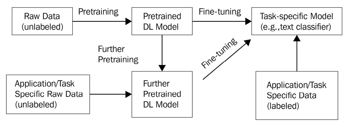
Let's walk through an example to understand a typical core DL development paradigm. For example, the popular BERT model released in late 2018 (a basic version of the BERT model can be found at https://huggingface.co/bert-base-uncased) was initially pretrained on raw texts (without human labeling) from over 11,000 books from BookCorpus and the entire English Wikipedia. This pretrained language model was then fine-tuned to many downstream NLP tasks, such as text classification and sentiment analysis, in different application domains such as movie review classifications by using labeled movie review data (https://huggingface.co/datasets/imdb). Note that sometimes, it might be necessary to further pretrain a foundation model (for example, BERT) within the application domain by using unlabeled data before fine-tuning to boost the final model performance in terms of accuracy. This core DL development paradigm is illustrated in Figure 1.1:
Figure 1.1 – A typical core DL development paradigm
Note that while Figure 1.1 represents a common development paradigm, not all of these steps are necessary for a specific application scenario. For example, you might only need to do fine-tuning using a publicly available pretrained DL model with your labeled application-specific data. Therefore, you don't need to do your own pretraining or carry out further pretraining using unlabeled data since other people or organizations have already done the pretraining step for you.
DL over Classical ML
Unlike classical ML model development, where, usually, a feature engineering step is required to extract and transform raw data into features to train an ML model such as decision tree or logistic regression, DL can learn the features automatically, which is especially attractive for modeling unstructured data such as texts, images, videos, audio, and speeches. DL is also called representational learning due to this characteristic. In addition to this, DL is usually data- and compute-intensive, requiring Graphics Process Units (GPUs), Tensor Process Units (TPU), or other types of computing hardware accelerators for at-scale training and inference. Explainability for DL models is also harder to implement, compared with traditional ML models, although recent progress has now made that possible.
Implementing a basic DL sentiment classifier
To set up the development of a basic DL sentiment classifier, you need to create a virtual environment in your local environment. Let's assume that you have miniconda installed. You can implement the following in your command-line prompt to create a new virtual environment called dl_model and install the PyTorch lightning-flash package so that the model can be built:
conda create -n dl_model python==3.8.10
conda activate dl_model
pip install lightning-flash[all]==0.5.0
pip pytorch-lightning==1.4.4 datasets==1.9.0
Depending on your local machine's memory, the preceding commands might take about 10 minutes to finish. You can verify the success of your installation by running the following command:
conda list | grep lightning
If you see output similar to the following, your installation was successful:
lightning-bolts     0.3.4                    pypi_0    pypi
lightning-flash     0.5.0                    pypi_0    pypi
pytorch-lightning   1.4.4                    pypi_0    pypi
Now you are ready to build your first DL model!
To begin building a DL model, complete the following steps:
- Import the necessary
torch and flash libraries, and import download_data, TextClassificationData, and TextClassifier from the flash subpackages:import torch
import flash
from flash.core.data.utils import download_data
from flash.text import TextClassificationData, TextClassifier
- To get the dataset for fine-tuning, use
download_data to download the imdb.zip file, which is the public domain binary sentiment classification (positive/negative) dataset from Internet Movie Database (IMDb) to a local data folder. The IMDb ZIP file contains three CSV files: train.csvvalid.csv test.csv
Each file contains two columns: review and sentiment. We then use TextClassificationData.from_csv to declare a datamodule variable that assigns the "review" to input_fields, and the "sentiment" to target_fields. Additionally, it assigns the train.csv file to train_file, the valid.csv file to val_file, and the test.csv file to the test_file properties of datamodule, respectively:
download_data("https://pl-flash-data.s3.amazonaws.com/imdb.zip", "./data/")
datamodule = TextClassificationData.from_csv(
    input_fields="review",
    target_fields="sentiment",
    train_file="data/imdb/train.csv",
    val_file="data/imdb/valid.csv",
    test_file="data/imdb/test.csv"
)
- Once we have the data, we can now perform fine-tuning using a foundation model. First, we declare
classifier_model by calling TextClassifier with a backbone assigned to prajjwal1/bert-tiny (which is a much smaller BERT-like pretrained model located in the Hugging Face model repository: https://huggingface.co/prajjwal1/bert-tiny). This means our model will be based on the bert-tiny model.
- The next step is to set up the trainer by defining how many epochs we want to run and how many GPUs we want to use to run them. Here,
torch.cuda.device_count() will return either 0 (no GPU) or 1 to N, where N is the maximum number of GPUs you can have in your running environment. Now we are ready to call trainer.finetune to train a binary sentiment classifier for the IMDb dataset:classifier_model = TextClassifier(backbone="prajjwal1/bert-tiny", num_classes=datamodule.num_classes)
trainer = flash.Trainer(max_epochs=3, gpus=torch.cuda.device_count())
trainer.finetune(classifier_model, datamodule=datamodule, strategy="freeze")
DL Fine-Tuning Time
Depending on your running environment, the fine-tuning step might take a couple of minutes on a GPU or around 10 minutes (if you're only using a CPU). You can reduce max_epochs=1 if you simply want to get a basic version of the sentiment classifier quickly.
- Once the fine-tuning step is complete, we will test the accuracy of the model by running
trainer.test():trainer.test()
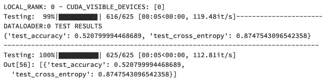
The output of the test should look similar to the following screenshot, whichindicates that the final model accuracy is about 52%:
Figure 1.2 – The test results of our first DL model
The test result shown in the preceding diagram indicates that we have a basic version of the model, as we only fine-tuned the foundation model for three epochs and haven't used any advanced techniques such as hyperparameter tuning or better fine-tuning strategies. However, this is a great accomplishment since you now have a working knowledge of how the core DL model paradigm works! We will explore more advanced model training techniques in later chapters of this book.
Understanding DL's full life cycle development
By now, you should have your first DL model ready and should feel proud of it. Now, let's explore the full DL life cycle together to fully understand its concepts, components, and challenges.
You might have gathered that the core DL development paradigm revolves around three key artifacts: Data, Model, and Code. In addition to this, Explainability is another major artifact that is required in many mission-critical application scenarios such as medical diagnoses, the financial industry, and decision making for criminal justice. As DL is usually considered a black box, providing explainability for DL increasingly becomes a key requirement before and after shipping to production.
Note that Figure 1.1 is still considered offline experimentation if we are still trying to figure out which model works using a dataset in a lab-like environment. Even in such an offline experimentation environment, things will quickly become complicated. Additionally, we would like to know and track which experiments we have or have not performed so that we don't waste time repeating the same experiments, whatever parameters and datasets we have used, and whatever kind of metrics we have for a specific model. Once we have a model that's good enough for the use cases and customer scenarios, the complexity increases as we need a way to continuously deploy and update the model in production, monitor the model and data drift, and then retrain the model when necessary. This complexity further increases when at-scale training, deployment, monitoring, and explainability are needed.
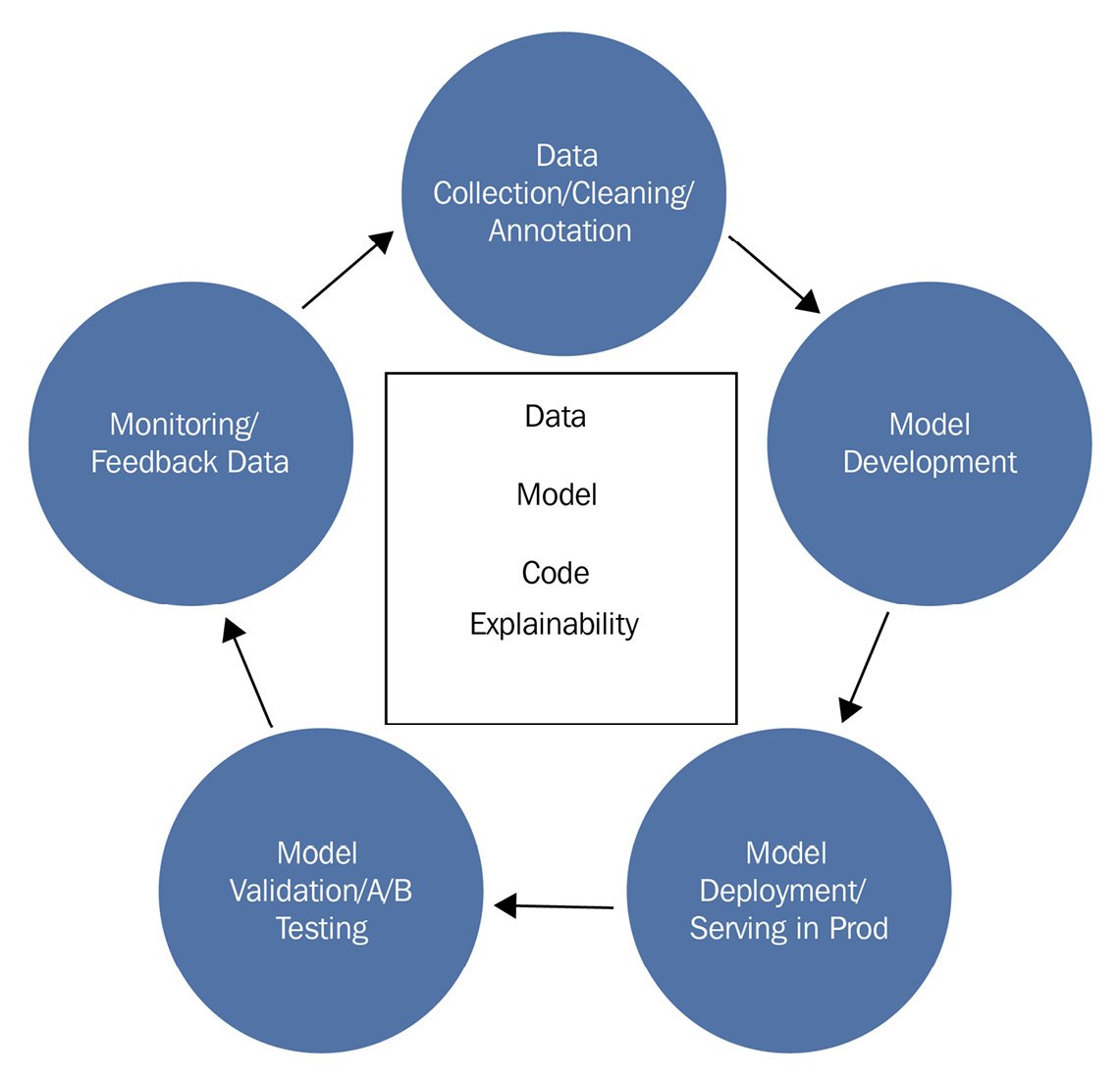
Let's examine what a DL life cycle looks like (see Figure 1.3). There are five stages:
- Data collection, cleaning, and annotation/labeling.
- Model development (which is also known as offline experimentation). The core DL development paradigm in Figure 1.1 is considered part of the model development stage, which itself can be an iterative process.
- Model deployment and serving in production.
- Model validation and A/B testing (which is also known as online experimentation; this is usually in a production environment).
- Monitoring and feedback data collection during production.
Figure 1.3 provides a diagram to show that it is a continuous development cycle for a DL model:
Figure 1.3 – The full DL development life cycle
In addition to this, we want to point out that the backbone of these five stages, as shown in Figure 1.3, essentially revolves around the four artifacts: data, model, code, and explainability. We will examine the challenges related to these four artifacts in the life cycle in the following sections. However, first, let's explore and understand MLOps, which is an evolving platform concept and framework that supports the full life cycle of ML. This will help us understand these challenges in a big-picture context.
Understanding MLOps challenges
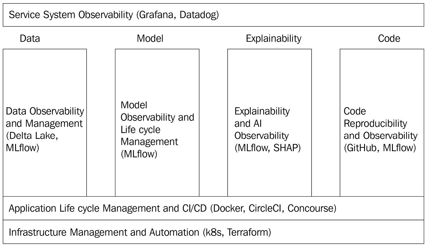
MLOps has some connections to DevOps, where a set of technology stacks and standard operational procedures are used for software development and deployment combined with IT operations. Unlike traditional software development, ML and especially DL represent a new era of software development paradigms called Software 2.0 (https://karpathy.medium.com/software-2-0-a64152b37c35). The key differentiator of Software 2.0 is that the behavior of the software does not just depend on well-understood programming language code (which is the characteristic of Software 1.0) but depends on the learned weights in a neural network that's difficult to write as code. In other words, there exists an inseparable integration of the code, data, and model that must be managed together. Therefore, MLOps is being developed and is still evolving to accommodate this new Software 2.0 paradigm. In this book, MLOps is defined as an operational automation platform that consists of three foundation layers and four pillars. They are listed as follows:
- Here are the three foundation layers:
- Infrastructure management and automation
- Application life cycle management and Continuous Integration and Continuous Deployment (CI/CD)
- Service system observability
- Here are the four pillars:
- Data observability and management
- Model observability and life cycle management
- Explainability and Artificial Intelligence (AI) observability
- Code reproducibility and observability
Additionally, we will explain MLflow's roles in these MLOps layers and pillars so that we have a clear picture regarding what MLflow can do to build up the MLOps layers in their entirety:
- Infrastructure management and automation: This includes, but is not limited to, Kubernetes (also known as k8s) for automated container orchestration and Terraform (commonly used for managing hundreds of cloud services and access control). These tools are adapted to manage ML and DL applications that have deployed models as service endpoints. These infrastructure layers are not the focus of this book; instead, we will focus on how to deploy a trained DL model using MLflow's provided capabilities.
- Application life cycle management and CI/CD: This includes, but is not limited to, Docker containers for virtualization, container life cycle management tools such as Kubernetes, and CircleCI or Concourse for CI and CD. Usually, CI means that whenever there are code or model changes in a GitHub repository, a series of automatic tests will be triggered to make sure no breaking changes are introduced. Once these tests have been passed, new changes will be automatically released as part of a new package. This will then trigger a new deployment process (CD) to deploy the new package to the production environment (often, this will include human approval as a safety gate). Note that these tools are not unique to ML applications but have been adapted to ML and DL applications, especially when we require GPU and distributed clusters for the training and testing of DL models. In this book, we will not focus on these tools but will mention the integration points or examples when needed.
- Service system observability: This is mostly for monitoring the hardware/clusters/CPU/memory/storage, operating system, service availability, latency, and throughput. This includes tools such as Grafana, Datadog, and more. Again, these are not unique to ML and DL applications and are not the focus of this book.
- Data observability and management: This is traditionally under-represented in the DevOps world but becomes very important in MLOps as data is critical within the full life cycle of ML/DL models. This includes data quality monitoring, outlier detection, data drift and concept drift detection, bias detection, secured and compliant data sharing, data provenance tracking and versioning, and more. The tool stacks in this area that are suitable for ML and DL applications are still emerging. A few examples include DataFold (https://www.datafold.com/) and Databand (https://databand.ai/open-source/). A recent development in data management is a unified lakehouse architecture and implementation called Delta Lake (http://delta.io) that can be used for ML data management. MLflow has native integration points with Delta Lake, and we will cover that integration in this book.
- Model observability and life cycle management: This is unique to ML/DL models, and it only became widely available recently due to the rise of MLflow. This includes tools for model training, testing, versioning, registration, deployment, serialization, model drift monitoring, and more. We will learn about the exciting capabilities that MLflow provides in this area. Note that once we combine CI/CD tools with MLflow training/monitoring, user feedback loops, and human annotations, we can achieve Continuous Training, Continuous Testing, and Continuous Labeling. MLflow provides the foundational capabilities so that further automation in MLOps becomes possible, although such complete automation will not be the focus of this book. Interested readers can find relevant references at the end of this chapter to explore this area further.
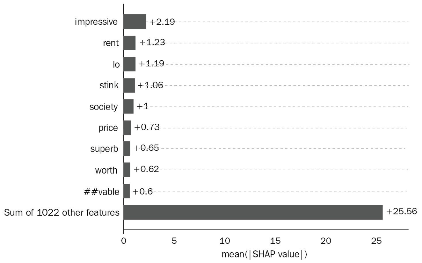
- Explainability and AI observability: This is unique to ML/DL models and is especially important for DL models, as traditionally, DL models are treated as black boxes. Understanding why the model provides certain predictions is critical for societally important applications. For example, in medical, financial, juridical, and many human-in-the-loop decision support applications, such as civilian and military emergency response, the demand for explainability is increasingly higher. MLflow provides native integration with a popular explainability framework called SHAP, which we will cover in this book.
- Code reproducibility and observability: This is not entirely unique to ML/DL applications. However, DL models face some special challenges as the number of DL code frameworks are diverse and the need to reproduce a model is not entirely up to the code alone (we also need data and execution environments such as GPU clusters). In addition to this, notebooks are commonly used in model development and production. How to manage the notebooks along with the model run is important. Usually, GitHub is used to manage the code repository; however, we need to structure the ML project code in a way that's reproducible either locally (such as on a local laptop) or remotely (for example, in a Databricks' GPU cluster). MLflow provides this capability to allow DL projects that have been written once to run anywhere, whether this is in an offline experimentation environment or an online production environment. We will cover MLflow's MLproject capability in this book.
In summary, MLflow plays a critical and foundational role in MLOps. It fills in the gaps that DevOps traditionally does not cover and, thus, is the focus of this book. The following diagram (Figure 1.4) shows the central roles of MLflow in the still-evolving MLOps world:
Figure 1.4 – The three layers and four pillars of MLOps and MLflow's roles
While the bottom two layers and the topmost layer are common within many software development and deployment processes, the middle four pillars are either entirely unique to ML/DL applications or partially unique to ML/DL applications. MLflow plays a critical role in all four of these pillars in MLOps. This book will help you to confidently apply MLflow to solve the issues of these four pillars while also equipping you to further integrate with other tools in the MLOps layers depicted in Figure 1.4 for full automation depending on your scenario requirements.
 Argentina
 Australia
 Austria
 Belgium
 Brazil
 Bulgaria
 Canada
 Chile
Chile
 Colombia
 Cyprus
 Czechia
 Denmark
 Ecuador
 Egypt
Egypt
 Estonia
 Finland
 France
 Germany
 Great Britain
 Greece
 Hungary
 India
India
 Indonesia
 Ireland
 Italy
Italy
 Japan
Japan
 Latvia
 Lithuania
 Luxembourg
 Malaysia
 Malta
Malta
 Mexico
 Netherlands
 New Zealand
 Norway
 Philippines
 Poland
 Portugal
 Romania
 Russia
 Singapore
 Slovakia
 Slovenia
 South Africa
 South Korea
 Spain
Spain
 Sweden
 Switzerland
 Taiwan
 Thailand
 Turkey
 Ukraine
 United States