

Introduction to Scikit-Learn
While pandas will save you a lot of time loading, examining, and cleaning data, the machine learning algorithms that will enable you to do predictive modeling are located in other packages. Scikit-learn is a foundational machine learning package for Python that contains many useful algorithms and has also influenced the design and syntax of other machine learning libraries in Python. For this reason, we focus on scikit-learn to develop skills in the practice of predictive modeling. While it's impossible for any one package to offer everything, scikit-learn comes pretty close in terms of accommodating a wide range of classic approaches for classification, regression, and unsupervised learning. However, it does not offer much functionality for some more recent advancements, such as deep learning.
Here are a few other related packages you should be aware of:
SciPy:
- Most of the packages we've used so far, such as NumPy and pandas, are actually part of the SciPy ecosystem.
- SciPy offers lightweight functions for classic methods such as linear regression and linear programming.
StatsModels:
- More oriented toward statistics and maybe more comfortable for users familiar with R
- Can get p-values and confidence intervals on regression coefficients
- Capability for time series models such as ARIMA
XGBoost and LightGBM:
- Offer a suite of state-of-the-art ensemble models that often outperform random forests. We will learn about XGBoost in Chapter 6, Gradient Boosting, SHAP Values, and Dealing with Missing Data.
TensorFlow, Keras, and PyTorch:
- Deep learning capabilities
There are many other Python packages that may come in handy, but this gives you an idea of what's out there.
Scikit-learn offers a wealth of different models for various tasks, but, conveniently, the syntax for using them is consistent. In this section, we will illustrate model syntax using a logistic regression model. Logistic regression, despite its name, is actually a classification model. This is one of the simplest, and therefore most important, classification models. In the next chapter, we will go through the mathematical details of how logistic regression works. Until then, you can simply think of it as a black box that can learn from labeled data, then make predictions.
From the first chapter, you should be familiar with the concept of training an algorithm on labeled data so that you can use this trained model to then make predictions on new data. Scikit-learn encapsulates these core functionalities in the .fit method for training models, and the .predict method for making predictions. Because of the consistent syntax, you can call .fit and .predict on any scikit-learn model from linear regression to classification trees.
The first step is to choose some model, in this example a logistic regression model, and instantiate it from the class provided by scikit-learn. In Python, classes are templates for creating objects, which are collections of functions, like .fit, and data, such as information learned from the model fitting process. When you instantiate a model class from scikit-learn, you are taking the blueprint of the model that scikit-learn makes available to you and creating a useful object out of it. You can train this object on your data and then save it to disk for later use. The following snippets can be used to perform this task. The first step is to import the class:
from sklearn.linear_model import LogisticRegression
The code to instantiate the class into an object is as follows:
my_lr = LogisticRegression()
The object is now a variable in our workspace. We can examine it using the following code:
my_lr
This should give the following output:
LogisticRegression()
Notice that the act of creating the model object involves essentially no knowledge of what logistic regression is or how it works. Although we didn't select any particular options when creating the logistic regression model object, we are now in fact using many default options for how the model is formulated and would be trained. In effect, these are choices we have made regarding the details of model implementation without having been aware of it. The danger of an easy-to-use package such as scikit-learn is that it has the potential to obscure these choices from you. However, any time you use a machine learning model that has been prepared for you as scikit-learn models have been, your first job is to understand all the options that are available. A best practice in such cases is to explicitly provide every keyword parameter to the model when you create the object. Even if you are just selecting all the default options, this will help increase your awareness of the choices that are being made.
We will review the interpretation of these choices later on, but for now here is the code for instantiating a logistic regression model with all the default options:
my_new_lr = LogisticRegression(penalty='l2', dual=False,\
                               tol=0.0001, C=1.0,\
                               fit_intercept=True,\
                               intercept_scaling=1,\
                               class_weight=None,\
                               random_state=None,\
                               solver='lbfgs',\
                               max_iter=100,\
                               multi_class='auto',\
                               verbose=0, warm_start=False,\
                               n_jobs=None, l1_ratio=None)
Even though the object we've created here in my_new_lr is identical to my_lr, being explicit like this is especially helpful when you are starting out and learning about different kinds of models. Once you're more comfortable, you may wish to just instantiate with the default options and make changes later as necessary. Here, we show how this may be done. The following code sets two options and displays the current state of the model object:
my_new_lr.C = 0.1
my_new_lr.solver = 'liblinear'
my_new_lr
This should produce the following:
Out[11]:LogisticRegression(C=0.1, solver='liblinear')
Notice that only the options we have updated from the default values are displayed. Here, we've taken what is called a hyperparameter of the model, C, and updated it from its default value of 1 to 0.1. We've also specified a solver. For now, it is enough to understand that hyperparameters are options that you supply to the model, before fitting it to the data. These options specify the way in which the model will be trained. Later, we will explain in detail what all the options are and how you can effectively choose values for them.
To illustrate the core functionality, we will fit this nearly default logistic regression to some data. Supervised learning algorithms rely on labeled data. That means we need both the features, customarily contained in a variable called X, and the corresponding responses, in a variable called y. We will borrow the first 10 samples of one feature, and the response, from our dataset to illustrate:
X = df['EDUCATION'][0:10].values.reshape(-1,1)
X
That should show the values of the EDUCATION feature for the first 10 samples:

Figure 2.2: First 10 values of a feature
The corresponding first 10 values of the response variable can be obtained as follows:
y = df['default payment next month'][0:10].values
y
Here is the output:
Out[13]: array([1, 1, 0, 0, 0, 0, 0, 0, 0, 0])
Here, we have selected a couple of Series (that is, columns) from our DataFrame: the EDUCATION feature we've been discussing, and the response variable. Then we selected the first 10 elements of each and finally used the .values method to return NumPy arrays. Also notice that we used the .reshape method to reshape the features. Scikit-learn expects that the first dimension (that is, the number of rows) of the array of features will be equal to the number of samples, so we need to make that reshaping for X, but not for y. The –1 in the first positional argument of .reshape means to make the output array shape flexible in that dimension, according to how much data goes in. Since we just have a single feature in this example, we specified the number of columns as the second argument, 1, and let the –1 argument indicate that the array should "fill up" along the first dimension with as many elements as necessary to accommodate the data, in this case, 10 elements. Note that while we've extracted the data into NumPy arrays to show how this can be done, it's also possible to use pandas Series as direct input to scikit-learn.
Let's now use this data to fit our logistic regression. This is accomplished with just one line:
my_new_lr.fit(X, y)
Here is the output:
Out[14]:LogisticRegression(C=0.1, solver='liblinear')
That's all there is to it. Once the data is prepared and the model is specified, fitting the model almost seems like an afterthought. Of course, we are ignoring all the important options and what they mean right now. But, technically speaking, fitting a model is very easy in terms of the code. You can see that the output of this cell just prints the same options we've already seen. While the fitting procedure did not return anything aside from this output, a very important change has taken place. The my_new_lr model object is now a trained model. We say that this change happened in place since no new object was created; the existing object, my_new_lr, has been modified. This is similar to modifying a DataFrame in place. We can now use our trained model to make predictions using the features of new samples, that the model has never "seen" before. Let's try the next 10 rows from the EDUCATION feature.
We can select and view these features using a new variable, new_X:
new_X = df['EDUCATION'][10:20].values.reshape(-1,1)
new_X

Figure 2.3: New features to make predictions for
Making predictions is done like this:
my_new_lr.predict(new_X)
Here is the output:
array([0, 0, 0, 0, 0, 0, 0, 0, 0, 0])
We can also view the true values corresponding to these predictions, since this data is labeled:
df['default payment next month'][10:20].values
Here is the output:
Out[17]:array([0, 0, 0, 1, 0, 0, 1, 0, 0, 0])
Here, we've illustrated several things. After getting our new feature values, we've called the .predict method on the trained model. Notice that the only argument to this method is a set of features, that is, an "X" that we've called new_X.
How well did our little model do? We may naively observe that since the model predicted all 0s, and 80% of the true labels are 0s, we were right 80% of the time, which seems pretty good. On the other hand, we entirely failed to successfully predict any 1s. So, if those were important, we did not actually do very well. While this is just an example to get you familiar with how scikit-learn works, it's worth considering what a "good" prediction might look like for this problem. We will get into the details of assessing model predictive capabilities shortly. For now, congratulate yourself on having gotten your hands dirty with some real data and fitting your first machine learning model.
Generating Synthetic Data
In the following exercise, you will walk through the model fitting process on your own. We’ll motivate this process using a linear regression, one of the best-known mathematical models, which should be familiar from basic statistics. It’s also called a line of best fit. If you don’t know what it is, you could consult a basic statistics resource, although the intent here is to illustrate the mechanics of model fitting in sci-kit learn, as opposed to understanding the model in detail. We’ll work on that later in the book for other mathematical models that we’ll apply to the case study, such as logistic regression. In order to have data to work with, you will generate your own synthetic data. Synthetic data is a valuable learning tool for exploring models, illustrating mathematical concepts, and for conducting thought experiments to test various ideas. In order to make synthetic data, we will again illustrate here how to use NumPy's random library to generate random numbers, as well as matplotlib's scatter and plot functions to create scatter and line plots. In the exercise, we'll use scikit-learn for the linear regression part.
To get started, we use NumPy to make a one-dimensional array of feature values, X, consisting of 1,000 random real numbers (in other words, not just integers but decimals as well) between 0 and 10. We again use a seed for the random number generator. Next, we use the .uniform method of default_rng (random number generator), which draws from the uniform distribution: it's equally likely to choose any number between low (inclusive) and high (exclusive), and will return an array of whatever size you specify. We create a one-dimensional array (that is, a vector) with 1,000 elements, then examine the first 10. All of this can be done using the following code:
from numpy.random import default_rng
rg = default_rng(12345)
X = rg.uniform(low=0.0, high=10.0, size=(1000,))
X[0:10]
The output should appear as follows:

Figure 2.4: Creating random, uniformly distributed numbers with NumPy
Data for Linear Regression
Now we need a response variable. For this example, we'll generate data that follows the assumptions of linear regression: the data will exhibit a linear trend against the feature, but have normally distributed errors:

Figure 2.5: Linear equation with Gaussian noise
Here, a is the slope, b is the intercept, and the Gaussian noise has a mean of µ with a standard deviation of σ. In order to write code to implement this, we need to make a corresponding vector of responses, y, which are calculated as the slope times the feature array, X, plus some Gaussian noise (again using NumPy), and an intercept. The noise will be an array of 1,000 data points with the same shape (size) as the feature array, X, where the mean of the noise (loc) is 0 and the standard deviation (scale) is 1. This will add a little "spread" to our linear data:
slope = 0.25
intercept = -1.25
y = slope * X + rg.normal(loc=0.0, scale=1.0, size=(1000,))\
          + intercept
Now we'd like to visualize this data. We will use matplotlib to plot y against the feature X as a scatter plot. First, we use .rcParams to set the resolution (dpi = dots per inch) for a nice crisp image. Then we create the scatter plot with plt.scatter, where X and y are the first two arguments, respectively, and the s argument specifies a size for the dots.
This code can be used for plotting:
mpl.rcParams['figure.dpi'] = 400
plt.scatter(X,y,s=1)
plt.xlabel('X')
plt.ylabel('y')
After executing these cells, you should see something like this in your notebook:
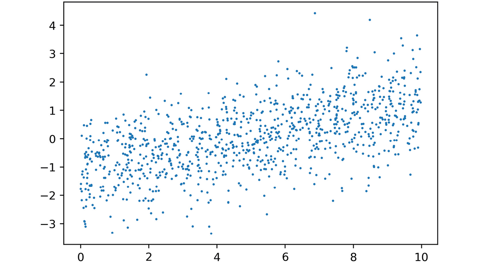
Figure 2.6: Plot the noisy linear relationship
Looks like some noisy linear data, just like we hoped. Now let's model it.
Note
If you're reading the print version of this book, you can download and browse the color versions of some of the images in this chapter by visiting the following link: https://packt.link/0dbUp.
Exercise 2.01: Linear Regression in Scikit-Learn
In this exercise, we will take the synthetic data we just generated and determine a line of best fit, or linear regression, using scikit-learn. The first step is to import a linear regression model class from scikit-learn and create an object from it. The import is similar to the LogisticRegression class we worked with previously. As with any model class, you should observe what all the default options are. Notice that for linear regression, there are not that many options to specify: you will use the defaults for this exercise. The default settings include fit_intercept=True, meaning the regression model will include an intercept term. This is certainly appropriate since we added an intercept to the synthetic data. Perform the following steps to complete the exercise, noting that the code creating the data for linear regression from the preceding section must be run first in the same notebook (as seen on GitHub):
Note
The Jupyter notebook for this exercise can be found here: https://packt.link/IaoyM.
- Execute this code to import the linear regression model class and instantiate it with all the default options:
from sklearn.linear_model import LinearRegression
lin_reg = LinearRegression(fit_intercept=True, normalize=False,\
                           copy_X=True, n_jobs=None)
lin_reg
You should see the following output:
Out[11]:LinearRegression()
No options are displayed since we used all the defaults. Now we can fit the model using our synthetic data, remembering to reshape the feature array (as we did earlier) so that that samples are along the first dimension. After fitting the linear regression model, we examine
lin_reg.intercept_, which contains the intercept of the fitted model, as well aslin_reg.coef_, which contains the slope. - Run this code to fit the model and examine the coefficients:
lin_reg.fit(X.reshape(-1,1), y)
print(lin_reg.intercept_)
print(lin_reg.coef_)
You should see this output for the intercept and slope:
-1.2522197212675905
[0.25711689]
We again see that actually fitting a model in scikit-learn, once the data is prepared and the options for the model are decided, is a trivial process. This is because all the algorithmic work of determining the model parameters is abstracted away from the user. We will discuss this process later, for the logistic regression model we'll use on the case study data.
What about the slope and intercept of our fitted model?
These numbers are fairly close to the slope and intercept we indicated when creating the model. However, because of the random noise, they are only approximations.
Finally, we can use the model to make predictions on feature values. Here, we do this using the same data used to fit the model: the array of features,
X. We capture the output of this as a variable,y_pred. This is very similar to the example shown in Figure 2.7, only here we are making predictions on the same data used to fit the model (previously, we made predictions on different data) and we put the output of the.predictmethod into a variable. - Run this code to make predictions:
y_pred = lin_reg.predict(X.reshape(-1,1))
We can plot the predictions,
y_pred, against featureXas a line plot over the scatter plot of the feature and response data, like we made in Figure 2.6. Here, we make the addition ofplt.plot, which produces a line plot by default, to plot the feature and the model-predicted response values for the model training data. Notice that we follow theXandydata with'r'in our call toplt.plot. This keyword argument causes the line to be red and is part of a shorthand syntax for plot formatting. - This code can be used to plot the raw data, as well as the fitted model predictions on this data:
plt.scatter(X,y,s=1)
plt.plot(X,y_pred,'r')
plt.xlabel('X')
plt.ylabel('y')
After executing this cell, you should see something like this:

Figure 2.7: Plotting the data and the regression line
The plot looks like a line of best fit, as expected.
In this exercise, as opposed to when we called .predict with logistic regression, we made predictions on the same data X that we used to train the model. This is an important distinction. While here, we are seeing how the model "fits" the same data that it was trained on, we previously examined model predictions on new, unseen data. In machine learning, we are usually concerned with predictive capabilities: we want models that can help us know the likely outcomes of future scenarios. However, it turns out that model predictions on both the training data used to fit the model and the test data, which was not used to fit the model, are important for understanding the workings of the model. We will formalize these notions later in Chapter 4, The Bias-Variance Trade-Off, when we discuss the bias-variance trade-off.