Linear Models – From Risk Factors to Return Forecasts

The family of linear models represents one of the most useful hypothesis classes. Many learning algorithms that are widely applied in algorithmic trading rely on linear predictors because they can be efficiently trained, are relatively robust to noisy financial data, and have strong links to the theory of finance. Linear predictors are also intuitive, easy to interpret, and often fit the data reasonably well or at least provide a good baseline.

Linear regression has been known for over 200 years, since Legendre and Gauss applied it to  astronomy and began to analyze its statistical properties. Numerous extensions have since adapted the linear regression model and the baseline ordinary least squares (OLS) method to learn its parameters:

• Generalized linear models (GLM) expand the scope of applications by allowing for response variables that imply an error distribution other than the normal distribution...

From inference to prediction

As the name suggests, linear regression models assume that the output is the result of a linear combination of the inputs. The model also assumes a random error that allows for each observation to deviate from the expected linear relationship. The reasons that the model does not perfectly describe the relationship between inputs and output in a deterministic way include, for example, missing variables, measurement, or data collection issues.

If we want to draw statistical conclusions about the true (but not observed) linear relationship in the population based on the regression parameters estimated from the sample, we need to add assumptions about the statistical nature of these errors. The baseline regression model makes the strong assumption that the distribution of the errors is identical across observations. It also assumes that errors are independent of each other—in other words, knowing one error does not help to forecast...

The baseline model – multiple linear regression

We will begin with the model's specification and objective function, the methods we can use to learn its parameters, and the statistical assumptions that allow the inference and diagnostics of these assumptions. Then, we will present extensions that we can use to adapt the model to situations that violate these assumptions. Useful references for additional background include Wooldridge (2002 and 2008).

How to formulate the model

The multiple regression model defines a linear functional relationship between one continuous outcome variable and p input variables that can be of any type but may require preprocessing. Multivariate regression, in contrast, refers to the regression of multiple outputs on multiple input variables.

In the population, the linear regression model has the following form for a single instance of the output y, an input vector , and the error :

The interpretation of the coefficients...

How to run linear regression in practice

The accompanying notebook, linear_regression_intro.ipynb, illustrates a simple and then a multiple linear regression, the latter using both OLS and gradient descent. For the multiple regression, we generate two random input variables x₁ and x₂ that range from -50 to +50, and an outcome variable that's calculated as a linear combination of the inputs, plus random Gaussian noise, to meet the normality assumption GMT 6:

OLS with statsmodels

We use statsmodels to estimate a multiple regression model that accurately reflects the data-generating process, as follows:

import statsmodels.api as sm
X_ols = sm.add_constant(X)
model = sm.OLS(y, X_ols).fit()
model.summary()

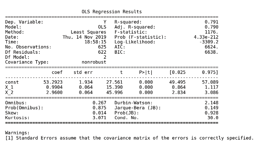
This yields the following OLS Regression Results summary:

Figure 7.2: OLS Regression Results summary

The upper part of the summary displays the dataset characteristics—namely, the estimation method and the number of observations and parameters...

How to build a linear factor model

Algorithmic trading strategies use factor models to quantify the relationship between the return of an asset and the sources of risk that are the main drivers of these returns. Each factor risk carries a premium, and the total asset return can be expected to correspond to a weighted average of these risk premia.

There are several practical applications of factor models across the portfolio management process, from construction and asset selection to risk management and performance evaluation. The importance of factor models continues to grow as common risk factors are now tradeable:

• A summary of the returns of many assets, by a much smaller number of factors, reduces the amount of data required to estimate the covariance matrix when optimizing a portfolio.
• An estimate of the exposure of an asset or a portfolio to these factors allows for the management of the resulting risk, for instance, by entering suitable hedges when risk...

Regularizing linear regression using shrinkage

The least-squares method to train a linear regression model will produce the best linear and unbiased coefficient estimates when the Gauss–Markov assumptions are met. Variations like GLS fare similarly well, even when OLS assumptions about the error covariance matrix are violated. However, there are estimators that produce biased coefficients to reduce the variance and achieve a lower generalization error overall (Hastie, Tibshirani, and Friedman 2009).

When a linear regression model contains many correlated variables, their coefficients will be poorly determined. This is because the effect of a large positive coefficient on the RSS can be canceled by a similarly large negative coefficient on a correlated variable. As a result, the risk of prediction errors due to high variance increases because this wiggle room for the coefficients makes the model more likely to overfit to the sample.

How to hedge against overfitting...

How to predict returns with linear regression

In this section, we will use linear regression with and without shrinkage to predict returns and generate trading signals.

First, we need to create the model inputs and outputs. To this end, we'll create features along the lines we discussed in Chapter 4, Financial Feature Engineering – How to Research Alpha Factors, as well as forward returns for various time horizons, which we will use as outcomes for the models.

Then, we will apply the linear regression models discussed in the previous section to illustrate their usage with statsmodels and sklearn and evaluate their predictive performance. In the next chapter, we will use the results to develop a trading strategy and demonstrate the end-to-end process of backtesting a strategy driven by a machine learning model.

Preparing model features and forward returns

To prepare the data for our predictive model, we need to:

• Select a universe of equities and...

Linear classification

The linear regression model discussed so far assumes a quantitative response variable. In this section, we will focus on approaches to modeling qualitative output variables for inference and prediction, a process that is known as classification and that occurs even more frequently than regression in practice.

Predicting a qualitative response for a data point is called classifying that observation because it involves assigning the observation to a category, or class. In practice, classification methods often predict probabilities for each of the categories of a qualitative variable and then use this probability to decide on the proper classification.

We could approach this classification problem by ignoring the fact that the output variable assumes discrete values, and then applying the linear regression model to try to predict a categorical output using multiple input variables. However, it is easy to construct examples where this method performs very...

Summary

In this chapter, we introduced the first of our machine learning models using the important baseline case of linear models for regression and classification. We explored the formulation of the objective functions for both tasks, learned about various training methods, and learned how to use the model for both inference and prediction.

We applied these new machine learning techniques to estimate linear factor models that are very useful to manage risks, assess new alpha factors, and attribute performance. We also applied linear regression and classification to accomplish the first predictive task of predicting stock returns in absolute and directional terms.

In the next chapter, we will put together what we have covered so far in the form of the machine learning for trading workflow. This process starts with sourcing and preparing the data about a specific investment universe and the computation of useful features, continues with the design and evaluation of machine...