Chapter 5. Bayesian Regression Models
In the previous chapter, we covered the theory of Bayesian linear regression in some detail. In this chapter, we will take a sample problem and illustrate how it can be applied to practical situations. For this purpose, we will use the
generalized linear model (GLM) packages in R. Firstly, we will give a brief introduction to the concept of GLM to the readers.
Generalized linear regression
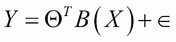
Recall that in linear regression, we assume the following functional form between the dependent variable Y and independent variable X:
Here, 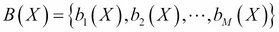 is a set of basis functions and
  is the parameter vector. Usually, it is assumed that
  , so
, so  represents an intercept or a bias term. Also, it is assumed that
  is a noise term distributed according to the normal distribution with mean zero and variance
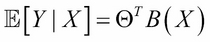
  . We also showed that this results in the following equation:
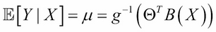
One can generalize the preceding equation to incorporate not only the normal distribution for noise but any distribution in the exponential family (reference 1 in the References section of this chapter). This is done by defining the following equation:
Here, g is called a link function. The well-known models, such as logistic regression, log-linear models, Poisson regression, and so on, are special cases of GLM. For example, in the case of ordinary linear regression, the link function would be  . For logistic regression...
In this chapter, for the purpose of illustrating Bayesian regression models, we will use the arm package of R. This package was developed by Andrew Gelman and co-workers, and it can be downloaded from the website at http://CRAN.R-project.org/package=arm.
The arm package has the bayesglm function that implements the Bayesian generalized linear model with an independent normal, t, or Cauchy prior distributions, for the model coefficients. We will use this function to build Bayesian regression models.
The Energy efficiency dataset
We will use the Energy efficiency dataset from the UCI Machine Learning repository for the illustration of Bayesian regression (reference 2 in the References section of this chapter). The dataset can be downloaded from the website at http://archive.ics.uci.edu/ml/datasets/Energy+efficiency. The dataset contains the measurements of energy efficiency of buildings with different building parameters. There are two energy efficiency parameters measured: heating load (Y1) and cooling load (Y2).
The building parameters used are: relative compactness (X1), surface area (X2), wall area (X3), roof area (X4), overall height (X5), orientation (X6), glazing area (X7), and glazing area distribution (X8). We will try to predict heating load as a function of all the building parameters using both ordinary regression and Bayesian regression, using the glm functions of the arm package. We will show that, for the same dataset, Bayesian regression gives significantly smaller prediction...
Regression of energy efficiency with building parameters
In this section, we will do a linear regression of the building's energy efficiency measure, heating load (Y1) as a function of the building parameters. It would be useful to do a preliminary descriptive analysis to find which building variables are statistically significant. For this, we will first create bivariate plots of Y1 and all the X variables. We will also compute the Spearman correlation between Y1 and all the X variables. The R script for performing these tasks is as follows:
Simulation of the posterior distribution
If one wants to find out the posterior of the model parameters, the sim( ) function of the arm package becomes handy. The following R script will simulate the posterior distribution of parameters and produce a set of histograms:
In this chapter, we illustrated how Bayesian regression is more useful for prediction with a tighter confidence interval using the Energy efficiency dataset and the bayesglm function of the arm package. We also learned how to simulate the posterior distribution using the sim function in the same R package. In the next chapter, we will learn about Bayesian classification.
 Argentina
 Australia
 Austria
 Belgium
 Brazil
 Bulgaria
 Canada
 Chile
Chile
 Colombia
 Cyprus
 Czechia
 Denmark
 Ecuador
 Egypt
Egypt
 Estonia
 Finland
 France
 Germany
 Great Britain
 Greece
 Hungary
 India
India
 Indonesia
 Ireland
 Italy
Italy
 Japan
Japan
 Latvia
 Lithuania
 Luxembourg
 Malaysia
 Malta
Malta
 Mexico
 Netherlands
 New Zealand
 Norway
 Philippines
 Poland
 Portugal
 Romania
 Russia
 Singapore
 Slovakia
 Slovenia
 South Africa
 South Korea
 Spain
Spain
 Sweden
 Switzerland
 Taiwan
 Thailand
 Turkey
 Ukraine
 United States