The transformer consists of a stack of  number of encoders. The output of one encoder is sent as input to the encoder above it. As shown in the following figure, we have a stack of number of encoders. Each encoder sends its output to the encoder above it. The final encoder returns the representation of the given source sentence as output. We feed the source sentence as input to the encoder and get the representation of the source sentence as output:
Figure 1.2 – A stack of N number of encoders
Note that in the transformer paper Attention Is All You Need, the authors have used  , meaning that they stacked up six encoders one above the another. However, we can try out different values of . For simplicity and better understanding, let's keep
  :
:
Figure 1.3 – A stack of encoders
Okay, the question is how exactly does the encoder work? How is it generating the representation for the given source sentence (input sentence)? To understand this, let's tap into the encoder and see its components. The following figure shows the components of the encoder:
Figure 1.4 – Encoder with its components
From the preceding figure, we can understand that all the encoder blocks are identical. We can also observe that each encoder block consists of two sublayers:
- Multi-head attention
- Feedforward network
Now, let's get into the details and learn how exactly these two sublayers works. To understand how multi-head attention works, first we need to understand the self-attention mechanism. So, in the next section, we will learn how the self-attention mechanism works.
Self-attention mechanism
Let's understand the self-attention mechanism with an example. Consider the following sentence:
A dog ate the food because it was hungry
In the preceding sentence, the pronoun it could mean either dog or food. By reading the sentence, we can easily understand that the pronoun it implies the dog and not food. But how does our model understand that in the given sentence, the pronoun it implies the dog and not food? Here is where the self-attention mechanism helps us.
In the given sentence, A dog ate the food because it was hungry, first, our model computes the representation of the word A, next it computes the representation of the word dog, then it computes the representation of the word ate, and so on. While computing the representation of each word, it relates each word to all other words in the sentence to understand more about the word.
For instance, while computing the representation of the word it, our model relates the word it to all the words in the sentence to understand more about the word it.
As shown in the following figure, in order to compute the representation of the word it, our model relates the word it to all the words in the sentence. By relating the word it to all the words in the sentence, our model can understand that the word it is related to the word dog and not food. As we can observe, the line connecting the word it to dog is thicker compared to the other lines, which indicates that the word it is related to the word dog and not food in the given sentence:
Figure 1.5 – Self-attention example
Okay, but how exactly does this work? Now that we have a basic idea of what the self-attention mechanism is, let's understand more about it in detail.
Suppose our input sentence (source sentence) is I am good. First, we get the embeddings for each word in our sentence. Note that the embeddings are just the vector representation of the word and the values of the embeddings will be learned during training.
Let 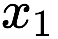 be the embedding of the word I,
 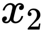 be the embedding of the word am, and
 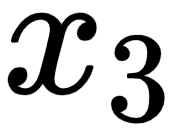 be the embedding of the word good. Consider the following:
- The embedding of the word I is
 .
.
- The embedding of the word am is
 .
.
- The embedding of the word good is
 .
.
Then, we can represent our input sentence I am good using the input matrix 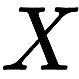 (embedding matrix or input embedding) as shown here:
Figure 1.6 – Input matrix
Note that the values used in the preceding matrix are arbitrary just to give us a better understanding.
From the preceding input matrix, 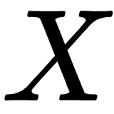 , we can understand that the first row of the matrix implies the embedding of the word I, the second row implies the embedding of the word am, and the third row implies the embedding of the word good. Thus, the dimension of the input matrix
 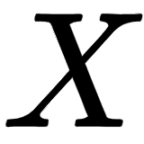 will be [sentence length x embedding dimension]. The number of words in our sentence (sentence length) is 3. Let the embedding dimension be 512; then, our input matrix (input embedding) dimension will be [3 x 512].
Now, from the input matrix, 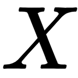 , we create three new matrices: a query matrix,
 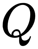 , key matrix,
 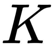 , and value matrix,
 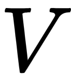 . Wait. What are these three new matrices? And why do we need them? They are used in the self-attention mechanism. We will see how exactly these three matrices are used in a while.
Okay, how we can create the query, key, and value matrices? To create these, we introduce three new weight matrices, called 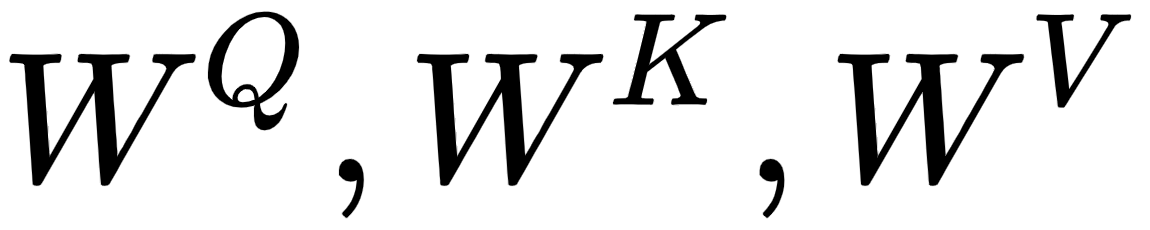 . We create the query, , key, , and value, , matrices by multiplying the input matrix,
 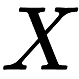 , by
, by 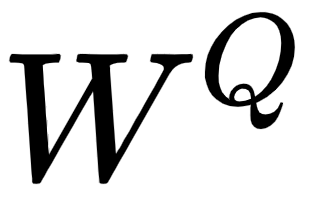 ,
, 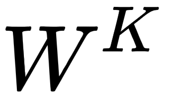 , and
, and 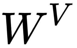 , respectively.
Note that the weight matrices, 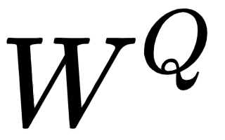 ,
,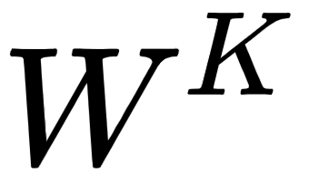 , and
, and 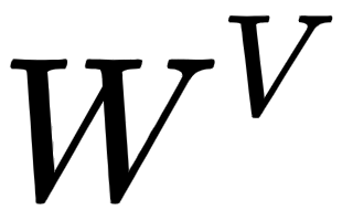 , are randomly initialized and their optimal values will be learned during training. As we learn the optimal weights, we will obtain more accurate query, key, and value matrices.
As shown in the following figure, multiplying the input matrix, 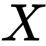 , by the weight matrices,
 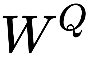 ,
,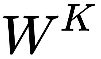 , and
, and 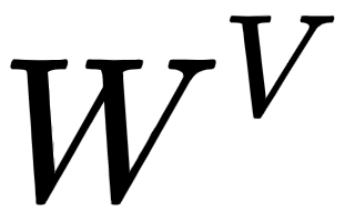 , we obtain the query, key, and value matrices:
Figure 1.7 – Creating query, key, and value matrices
From the preceding figure, we can understand the following:
- The first row in the query, key, and value matrices –
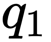 ,
, 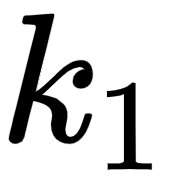 , and
, and 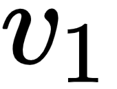 – implies the query, key, and value vectors of the word I.
- The second row in the query, key, and value matrices –
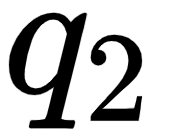 ,
, 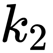 , and
, and 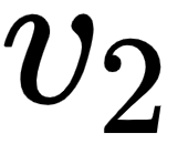 – implies the query, key, and value vectors of the word am.
- The third row in the query, key, and value matrices –
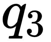 ,
, 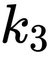 , and
, and 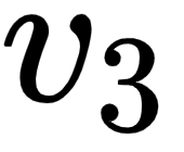 – implies the query, key, and value vectors of the word good.
Note that the dimensionality of the query, key, value vectors are 64. Thus, the dimension of our query, key, and value matrices is [sentence length x 64]. Since we have three words in the sentence, the dimensions of the query, key, and value matrices are [3 x 64].
But still, the ultimate question is why are we computing this? What is the use of query, key, and value matrices? How is this going to help us? This is exactly what we will discuss in detail in the next section.
Understanding the self-attention mechanism
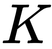
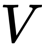
We learned how to compute query, 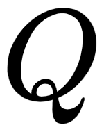 , key,
  , and value,
  , matrices and we also learned that they are obtained from the input matrix,
 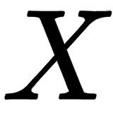 . Now, let's see how the query, key, and value matrices are used in the self-attention mechanism.
We learned that in order to compute a representation of a word, the self-attention mechanism relates the word to all the words in the given sentence. Consider the sentence I am good. To compute the representation of the word I, we relate the word I to all the words in the sentence, as shown in the following figure:
Figure 1.8 – Self-attention example
But why do we need to do this? Understanding how a word is related to all the words in the sentence helps us to learn better representation. Now, let's learn how the self-attention mechanism relates a word to all the words in the sentence using the query, key, and value matrices. The self-attention mechanism includes four steps; let's take a look at them one by one.
Step 1
The first step in the self-attention mechanism is to compute the dot product between the query matrix, 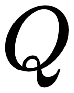 , and the key matrix,
 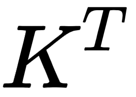 :
:
Figure 1.9 – Query and key matrices
The following shows the result of the dot product between the query matrix, 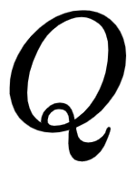 , and the key matrix,
 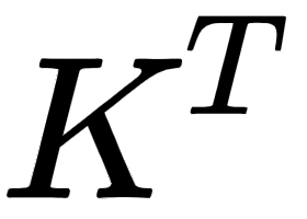 :
:
Figure 1.10 – Computing the dot product between the query and key matrices
But what is the use of computing the dot product between the query and key matrices? What exactly does 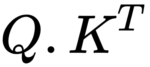 signify? Let's understand this by looking at the result of in detail.
Let's look into the first row of the matrix as shown in the following figure. We can observe that we are computing the dot product between the query vector 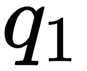 (I), and all the key vectors –
 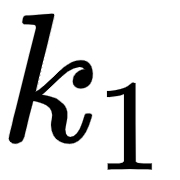 (I),
(I), 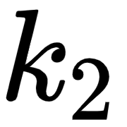 (am), and
 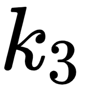 (good). Computing the dot product between two vectors tells us how similar they are.
Thus, computing the dot product between the query vector (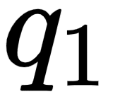 ) and the key vectors
 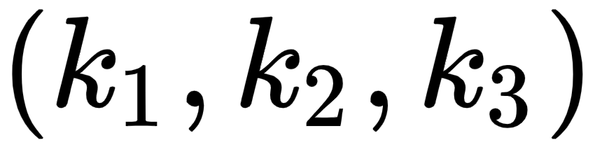 tells us how similar the query vector (I) is to all the key vectors – (I), (am), and (good). By looking at the first row of the matrix, we can understand that the word I is more related to itself than the words am and good since the dot product value is higher for
 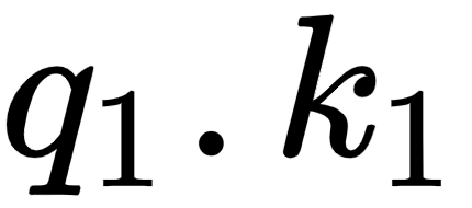 compared to
 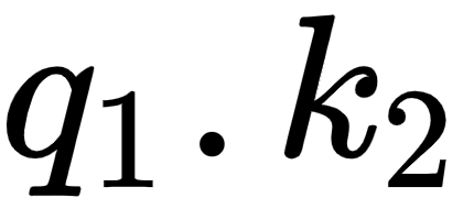 and
and 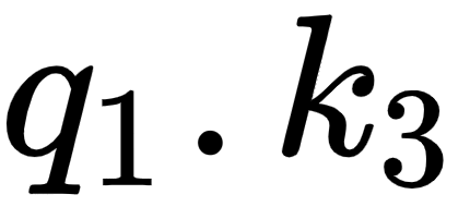 :
:
Figure 1.11 – Computing the dot product between the query vector (q1) and the key vectors (k1, k2, and k3)
Note that the values used in this chapter are arbitrary just to give us a better understanding.
Now, let's look into the second row of the matrix . As shown in the following figure, we can observe that we are computing the dot product between the query vector, 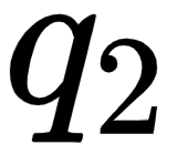 (am), and all the key vectors – (I), (am), and (good). This tells us how similar the query vector
 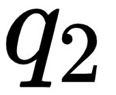 (am) is to the key vectors – (I), (am), and (good).
By looking at the second row of the matrix, we can understand that the word am is more related to itself than the words I and good since the dot product value is higher for 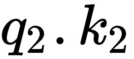 compared to
 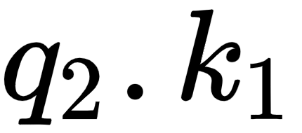 and
and 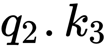 :
:
Figure 1.12 – Computing dot product between the query vector (q2) and the key vectors (k1, k2, and k3)
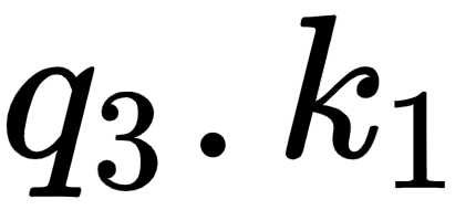
Similarly, let's look into the third row of the matrix. As shown in the following figure, we can observe that we are computing the dot product between the query vector 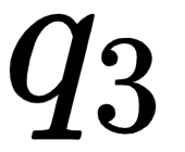 (good) and all the key vectors – (I), (am), and (good). This tells us how similar the query vector
 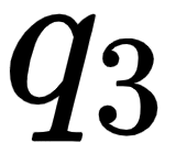 (good) is to all the key vectors – (I), (am), and (good).
By looking at the third row of the matrix, we can understand that the word good is more related to itself than the words I and am in the sentence since the dot product value is higher for 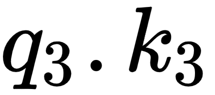 compared to
  and
and 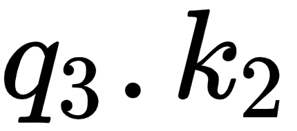 :
:
Figure 1.13 – Computing the dot product between the query vector (q3) and the key vectors (k1, k2, and k3)
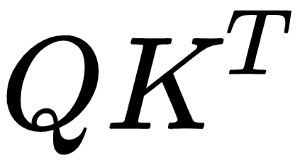
Thus, we can say that computing the dot product between the query matrix, , and the key matrix, , essentially gives us the similarity score, which helps us to understand how similar each word in the sentence is to all other words.
Step 2
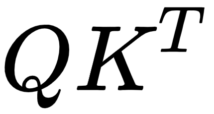
The next step in the self-attention mechanism is to divide the matrix by the square root of the dimension of the key vector. But why do we have to do that? This is useful in obtaining stable gradients.
Let 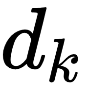 be the dimension of the key vector. Then, we divide by
 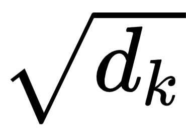 . The dimension of the key vector is 64. So, taking the square root of it, we will obtain 8. Hence, we divide Q.KT by 8 as shown in the following figure:
Figure 1.14 – Dividing Q.KT by the square root of dk
Step 3
By looking at the preceding similarity scores, we can understand that they are in the unnormalized form. So, we normalize them using the softmax function. Applying softmax function helps in bringing the score to the range of 0 to 1 and the sum of the scores equals to 1, as shown in the following figure:
Figure 1.15 – Applying the softmax function
We can call the preceding matrix a score matrix. With the help of these scores, we can understand how each word in the sentence is related to all the words in the sentence. For instance, look at the first row in the preceding score matrix; it tells us that the word I is related to itself by 90%, to the word am by 7%, and to the word good by 3%.
Step 4
Okay, what's next? We computed the dot product between the query and key matrices, obtained the scores, and then normalized the scores with the softmax function. Now, the final step in the self-attention mechanism is to compute the attention matrix, 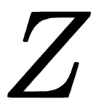 .
.
The attention matrix contains the attention values for each word in the sentence. We can compute the attention matrix, , by multiplying the score matrix, 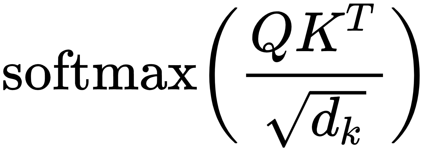 , by the value matrix,
 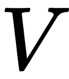 , as shown in the following figure:
Figure 1.16 – Computing the attention matrix
Say we have the following:
Figure 1.17 – Result of the attention matrix
The attention matrix, , is computed by taking the sum of the value vectors weighted by the scores. Let's understand this by looking at it row by row. First, let's see how for the first row, 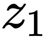 , the self-attention of the word I is computed:
Figure 1.18 – Self-attention of the word I
From the preceding figure, we can understand that 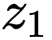 , the self-attention of the word I is computed as the sum of the value vectors weighted by the scores. Thus, the value of
 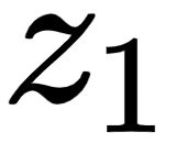 will contain 90% of the values from the value vector
 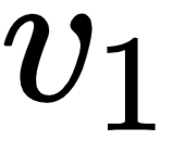 (I), 7% of the values from the value vector
 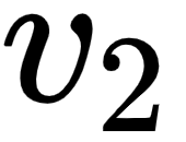 (am), and 3% of values from the value vector
 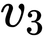 (good).
But how is this useful? To answer this question, let's take a little detour to the example sentence we saw earlier, A dog ate the food because it was hungry. Here, the word it indicates dog. To compute the self-attention of the word it, we follow the same preceding steps. Suppose we have the following:
Figure 1.19 – Self-attention of the word it
From the preceding figure, we can understand that the self-attention value of the word it contains 100% of the values from the value vector 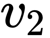 (dog). This helps the model to understand that the word it actually refers to dog and not food. Thus, by using a self-attention mechanism, we can understand how a word is related to all other words in the sentence.
Now, coming back to our example, 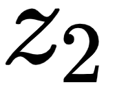 , the self-attention of the word am is computed as the sum of the value vectors weighted by the scores, as shown in the following figure:
Figure 1.20 – Self-attention of the word am
As we can observe from the preceding figure, the value of 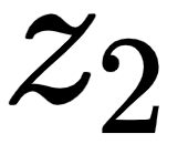 will contain 2.5% of the values from the value vector (I), 95% of the values from the value vector (am), and 2.5% of the values from the value vector
 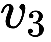 (good).
Similarly, 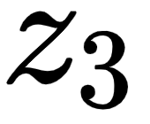 , the self-attention of the word good is computed as the sum of the value vectors weighted by the scores, as shown in the following figure:
Figure 1.21 – Self-attention of the word good
This implies that the value of 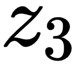 will contain 21% of the values from the value vector v1(I), 3% of the values from the value vector v2(am), and 76% of values from the value vector v3(good).
Thus, the attention matrix, , consists of self-attention values of all the words in the sentence and it is computed as follows:
To get a better understanding of the self-attention mechanism, the steps involved are summarized as follows:
- First, we compute the dot product between the query matrix and the key matrix,
 , and get the similarity scores.
- Next, we divide
 by the square root of the dimension of the key vector,
 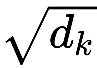 .
.
- Then, we apply the softmax function to normalize the scores and obtain the score matrix,
 .
.
- At the end, we compute the attention matrix,
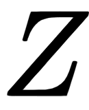 , by multiplying the score matrix by the value matrix,
 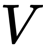 .
.
The self-attention mechanism is graphically shown as follows:
Figure 1.22 – Self-attention mechanism
The self-attention mechanism is also called scaled dot product attention, since here we are computing the dot product (between the query and key vectors) and scaling the values (with 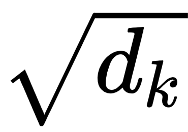 ).
).
Now that we have understood how the self-attention mechanism works, in the next section, we will learn about the multi-head attention mechanism.
Multi-head attention mechanism
Instead of having a single attention head, we can use multiple attention heads. That is, in the previous section, we learned how to compute the attention matrix, 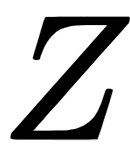 . Instead of computing a single attention matrix, , we can compute multiple attention matrices. But what is the use of computing multiple attention matrices?
Let's understand this with an example. Consider the phrase All is well. Say we need to compute the self-attention of the word well. After computing the similarity score, suppose we have the following:
Figure 1.23 – Self-attention of the word well
As we can observe from the preceding figure, the self-attention value of the word well is the sum of the value vectors weighted by the scores. If you look at the preceding figure closely, the attention value of the actual word well is dominated by the other word All. That is, since we are multiplying the value vector of the word All by 0.6 and the value vector of the actual word well by only 0.4, it implies that 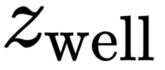 will contain 60% of the values from the value vector of the word All and only 40% of the values from the value vector of the actual word well. Thus, here the attention value of the actual word well is dominated by the other word All.
This will be useful only in circumstances where the meaning of the actual word is ambiguous. That is, consider the following sentence:
A dog ate the food because it was hungry
Say we are computing the self-attention for the word it. After computing the similarity score, suppose we have the following:
Figure 1.24 – Self-attention of the word it
As we can observe from the preceding equation, here the attention value of the word it is just the value vector of the word dog. Here, the attention value of the actual word it is dominated by the word dog. But this is fine here since the meaning of the word it is ambiguous as it may refer to either dog or food.
Thus, if the value vector of other words dominates the actual word in cases as shown in the preceding example, where the actual word is ambiguous, then this dominance is useful; otherwise, it will cause an issue in understanding the right meaning of the word. So, in order to make sure that our results are accurate, instead of computing a single attention matrix, we will compute multiple attention matrices and then concatenate their results. The idea behind using multi-head attention is that instead of using a single attention head, if we use multiple attention heads, then our attention matrix will be more accurate. Let's explore this in more detail.
Let's suppose we are computing two attention matrices, 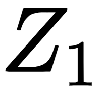 and
and 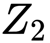 . First, let's compute the attention matrix
 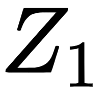 .
.
We learned that to compute the attention matrix, we create three new matrices, called query, key, and value matrices. To create the query, 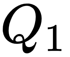 , key,
 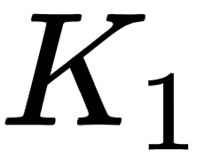 , and value,
 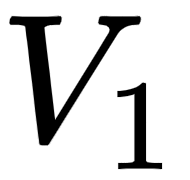 , matrices, we introduce three new weight matrices, called
 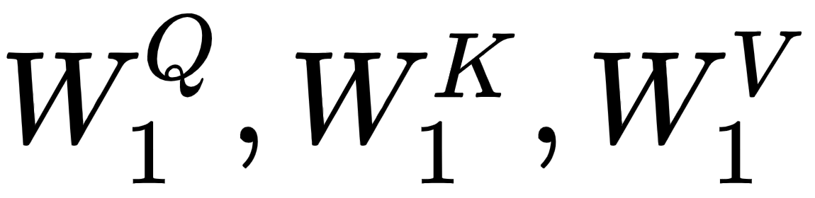 . We create the query, key, and value matrices by multiplying the input matrix, , by
 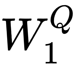 ,
,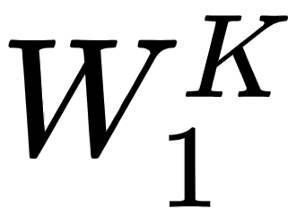 , and
, and 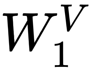 , respectively.
Now, the attention matrix 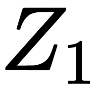 can be computed as follows:
Now, let's compute the second attention matrix, 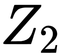 .
.
To compute the attention matrix , we create another set of query, Q2, key, K2, and value, V2, matrices. We introduce three new weight matrices, called 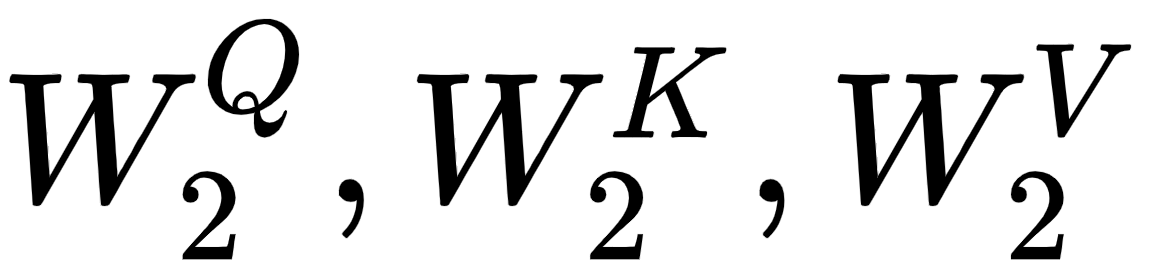 , and we create the query, key, and value matrices by multiplying the input matrix, , by
 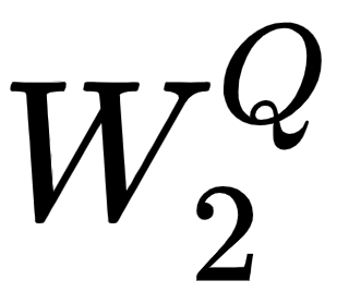 ,
,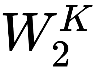 , and
, and 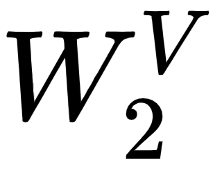 , respectively.
The attention matrix can be computed as follows:
Similarly, we can compute 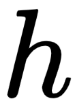 number of attention matrices. Suppose we have eight attention matrices,
 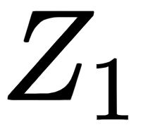 to
to 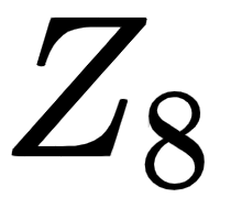 ; then, we can just concatenate all the attention heads (attention matrices) and multiply the result by a new weight matrix,
 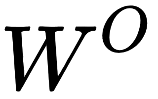 , and create the final attention matrix as shown:
Now that we have learned how the multi-attention mechanism works, we will learn about another interesting concept, called positional encoding, in the next section.
Learning position with positional encoding
Consider the input sentence I am good. In RNNs, we feed the sentence to the network word by word. That is, first the word I is passed as input, next the word am is passed, and so on. We feed the sentence word by word so that our network understands the sentence completely. But with the transformer network, we don't follow the recurrence mechanism. So, instead of feeding the sentence word by word, we feed all the words in the sentence parallel to the network. Feeding the words in parallel helps in decreasing the training time and also helps in learning the long-term dependency.
However, the problem is since we feed the words parallel to the transformer, how will it understand the meaning of the sentence if the word order is not retained? To understand the sentence, the word order (position of the words in the sentence) is important, right? Yes, the word order is very important as it helps to understand the position of each word in a sentence, which in turn helps to understand the meaning of the sentence.
So, we should give some information about the word order to the transformer so that it can understand the sentence. How can we do that? Let's explore this in more detail now.
For our given sentence, I am good, first, we get the embeddings for each word in our sentence. Let's represent the embedding dimension as 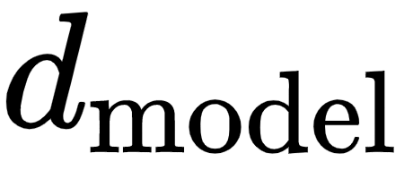 . Say the embedding dimension,
 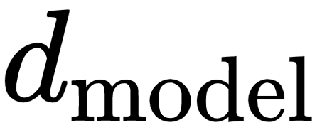 , is 4. Then, our input matrix dimension will be [sentence length x embedding dimension] = [3 x 4].
We represent our input sentence I am good using the input matrix (embedding matrix). Let the input matrix be the following:
Figure 1.25 – Input matrix
Now, if we pass the preceding input matrix 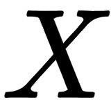 directly to the transformer, it cannot understand the word order. So, instead of feeding the input matrix directly to the transformer, we need to add some information indicating the word order (position of the word) so that our network can understand the meaning of the sentence. To do this, we introduce a technique called positional encoding. Positional encoding, as the name suggests, is an encoding indicating the position of the word in a sentence (word order).
The dimension of the positional encoding matrix, 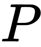 , is the same dimension as the input matrix
 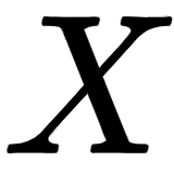 . Now, before feeding the input matrix (embedding matrix) to the transformer directly, we include the positional encoding. So, we simply add the positional encoding matrix
 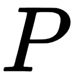 to the embedding matrix and then feed it as input to the network. So, now our input matrix will have not only the embedding of the word but also the position of the word in the sentence:
Figure 1.26 – Adding an input matrix and positional encoding matrix
Now, the ultimate question is how exactly is the positional encoding matrix computed? The authors of the transformer paper Attention Is All You Need have used the sinusoidal function for computing the positional encoding, as shown:
In the preceding equation, 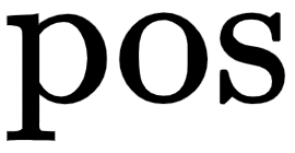 implies the position of the word in a sentence, and
 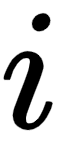 implies the position of the embedding. Let's understand the preceding equations with an example. By using the preceding equations, we can write the following:
Figure 1.27 – Computing the positional encoding matrix
As we can observe from the preceding matrix, in the positional encoding, we use the sin function when 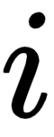 is even and the cos function when
 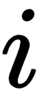 is odd. Simplifying the preceding matrix, we can write the following:
Figure 1.28 – Computing the positional encoding matrix
We know that in our input sentence, the word I is at the 0th position, am is at the 1st position, and good is at the 2nd position. Substituting the value, we can write the following:
Figure 1.29 – Computing the positional encoding matrix
Thus, our final positional encoding matrix, 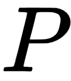 , is given as follows:
Figure 1.30 – Positional encoding matrix
After computing the positional encoding 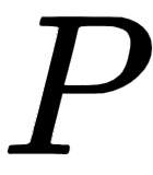 we simply perform element-wise addition with the embedding matrix
 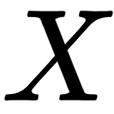 and feed the modified input matrix to the encoder.
Now, let's revisit our encoder architecture. A single encoder block is shown in the following figure. As we can observe, before feeding the input directly to the encoder, first, we get the input embedding (embedding matrix), and then we add the positional encoding to it, and then we feed it as input to the encoder:
Figure 1.31 – A single encoder block
We learned how the positional encoder works; we also learned how the multi-head attention sublayer works in the previous section. In the next section, we will learn how the feedforward network sublayer works in the encoder.
Feedforward network
The feedforward network sublayer in an encoder block is shown in the following figure:
Figure 1.32 – Encoder block
The feedforward network consists of two dense layers with ReLU activations. The parameters of the feedforward network are the same over the different positions of the sentence and different over the encoder blocks. In the next section, we will look into another interesting component of the encoder.
Add and norm component
One more important component in our encoder is the add and norm component. It connects the input and output of a sublayer. That is, as shown in the following figure (dotted lines), we can observe that the add and norm component:
- Connects the input of the multi-head attention sublayer to its output
- Connects the input of the feedforward sublayer to its output:
Figure 1.33 – Encoder block with the add and norm component
The add and norm component is basically a residual connection followed by layer normalization. Layer normalization promotes faster training by preventing the values in each layer from changing heavily.
Now that we have learned about all the components of the encoder, let's put all of them together and see how the encoder works as a whole in the next section.
Putting all the encoder components together
The following figure shows the stack of two encoders; only encoder 1 is expanded to reduce the clutter:
Figure 1.34 – A stack of encoders with encoder 1 expanded
From the preceding figure, we can understand the following:
- First, we convert our input to an input embedding (embedding matrix), and then add the position encoding to it and feed it as input to the bottom-most encoder (encoder 1).
- Encoder 1 takes the input and sends it to the multi-head attention sublayer, which returns the attention matrix as output.
- We take the attention matrix and feed it as input to the next sublayer, which is the feedforward network. The feedforward network takes the attention matrix as input and returns the encoder representation as output.
- Next, we take the output obtained from encoder 1 and feed it as input to the encoder above it (encoder 2).
- Encoder 2 carries the same process and returns the encoder representation of the given input sentence as output.
We can stack 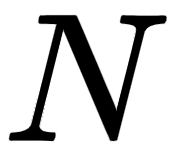 number of encoders one above the other; the output (encoder representation) obtained from the final encoder (topmost encoder) will be the representation of the given input sentence. Let's denote the encoder representation obtained from the final encoder (in our example, it is encoder 2) as
 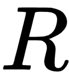 .
.
We take this encoder representation, 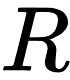 , obtained from the final encoder (encoder 2) and feed it as input to the decoder. The decoder takes the encoder representation
 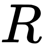 as input and tries to generate the target sentence.
Now that we have understood the encoder part of the transformer, in the next section, we will learn how a decoder works in detail.


 United States

 Great Britain
 India
India
 Germany
 France
 Canada
 Russia
 Spain
Spain
 Brazil
 Australia
 Singapore
 Canary Islands
 Hungary
 Ukraine
 Luxembourg
 Estonia
 Lithuania
 South Korea
 Turkey
 Switzerland
 Colombia
 Taiwan
 Chile
Chile
 Norway
 Ecuador
 Indonesia
 New Zealand
 Cyprus
 Denmark
 Finland
 Poland
 Malta
Malta
 Czechia
 Austria
 Sweden
 Italy
Italy
 Egypt
Egypt
 Belgium
 Portugal
 Slovenia
 Ireland
 Romania
 Greece
 Argentina
 Netherlands
 Bulgaria
 Latvia
 South Africa
 Malaysia
 Japan
Japan
 Slovakia
 Philippines
 Mexico
 Thailand






















 Filter