Search icon CANCEL
Subscription
0
Cart icon
Your Cart (0 item)
Close icon
You have no products in your basket yet
Arrow left icon
Explore Products
Best Sellers
New Releases
Books
Events
Videos
Audiobooks
Packt Hub
Free Learning
Arrow right icon
timer SALE ENDS IN
0 Days
:
00 Hours
:
00 Minutes
:
00 Seconds
Artificial Intelligence By Example

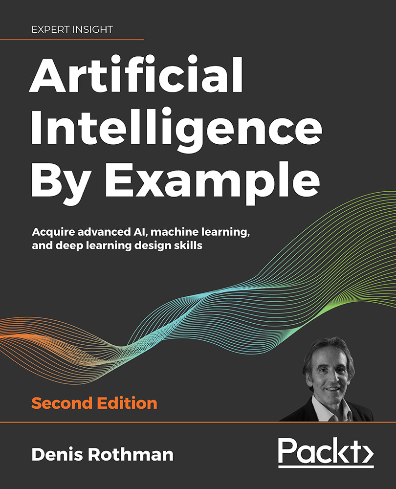
Artificial Intelligence By Example: Acquire advanced AI, machine learning, and deep learning design skills , Second Edition

eBook
$27.89 $30.99
Paperback
$45.99
eBook + Subscription
$29.99 Monthly

What do you get with eBook?

Product feature icon Instant access to your Digital eBook purchase
Product feature icon Download this book in EPUB and PDF formats
Product feature icon Access this title in our online reader with advanced features
Product feature icon DRM FREE - Read whenever, wherever and however you want
Product feature icon AI Assistant (beta) to help accelerate your learning
Modal Close icon
Payment Processing...
tick Completed

Billing Address

Table of content icon View table of contents Preview book icon Preview Book

Artificial Intelligence By Example

Building a Reward Matrix – Designing Your Datasets

Experimenting and implementation comprise the two main approaches of artificial intelligence. Experimenting largely entails trying ready-to-use datasets and black box, ready-to-use Python examples. Implementation involves preparing a dataset, developing preprocessing algorithms, and then choosing a model, the proper parameters, and hyperparameters.

Implementation usually involves white box work that entails knowing exactly how an algorithm works and even being able to modify it.

In Chapter 1, Getting Started with Next-Generation Artifcial Intelligence through Reinforcement Learning, the MDP-driven Bellman equation relied on a reward matrix. In this chapter, we will get our hands dirty in a white box process to create that reward matrix.

An MDP process cannot run without a reward matrix. The reward matrix determines whether it is possible to go from one cell to another, from A to B. It is like a map of a city that tells you if you are allowed to take a street or if it is a one-way street, for example. It can also set a goal, such as a place that you would like to visit in a city, for example.

To achieve the goal of designing a reward matrix, the raw data provided by other systems, software, and sensors needs to go through preprocessing. A machine learning program will not provide efficient results if the data has not gone through a standardization process.

The reward matrix, R, will be built using a McCulloch-Pitts neuron in TensorFlow. Warehouse management has grown exponentially as e-commerce has taken over many marketing segments. This chapter introduces automated guided vehicles (AGVs), the equivalent of an SDC in a warehouse to store and retrieve products.

The challenge in this chapter will be to understand the preprocessing phase in detail. The quality of the processed dataset will influence directly the accuracy of any machine learning algorithm.

This chapter covers the following topics:

  • The McCulloch-Pitts neuron will take the raw data and transform it
  • Logistic classifiers will begin the neural network process
  • The logistic sigmoid will squash the values
  • The softmax function will normalize the values
  • The one-hot function will choose the target for the reward matrix
  • An example of AGVs in a warehouse

The topics form a list of tools that, in turn, form a pipeline that will take raw data and transform it into a reward matrix—an MDP.

Designing datasets – where the dream stops and the hard work begins

As in the previous chapter, bear in mind that a real-life project goes through a three-dimensional method in some form or other. First, it's important to think and talk about the problem in need of solving without jumping onto a laptop. Once that is done, bear in mind that the foundation of machine learning and deep learning relies on mathematics. Finally, once the problem has been discussed and mathematically represented, it is time to develop the solution.

First, think of a problem in natural language. Then, make a mathematical description of a problem. Only then should you begin the software implementation.

Designing datasets

The reinforcement learning program described in the first chapter can solve a variety of problems involving unlabeled classification in an unsupervised decision-making process. The Q function can be applied to drone, truck, or car deliveries. It can also be applied to decision making in games or real life.

However, in a real-life case study problem (such as defining the reward matrix in a warehouse for the AGV, for example), the difficulty will be to produce an efficient matrix using the proper features.

For example, an AGV requires information coming from different sources: daily forecasts and real-time warehouse flows.

The warehouse manages thousands of locations and hundreds of thousands of inputs and outputs. Trying to fit too many features into the model would be counterproductive. Removing both features and worthless data requires careful consideration.

A simple neuron can provide an efficient way to attain the standardization of the input data.

Machine learning and deep learning are frequently used to preprocess input data for standardization purposes, normalization, and feature reduction.

Using the McCulloch-Pitts neuron

To create the reward matrix, R, a robust model for processing the inputs of the huge volumes in a warehouse must be reduced to a limited number of features.

In one model, for example, the thousands to hundreds of thousands of inputs can be described as follows:

  • Forecast product arrivals with a low priority weight: w1 = 10
  • Confirmed arrivals with a high priority weight: w2 = 70
  • Unplanned arrivals decided by the sales department: w3 = 75
  • Forecasts with a high priority weight: w4 = 60
  • Confirmed arrivals that have a low turnover and so have a low weight: w5 = 20

The weights have been provided as constants. A McCulloch-Pitts neuron does not modify weights. A perceptron neuron does as we will see beginning with Chapter 8, Solving the XOR Problem with a Feedforward Neural Network. Experience shows that modifying weights is not always necessary.

These weights form a vector, as shown here:

Each element of the vector represents the weight of a feature of a product stored in optimal locations. The ultimate phase of this process will produce a reward matrix, R, for an MDP to optimize itineraries between warehouse locations.

Let's focus on our neuron. These weights, used through a system such as this one, can attain up to more than 50 weights and parameters per neuron. In this example, 5 weights are implemented. However, in real-life case, many other parameters come into consideration, such as unconfirmed arrivals, unconfirmed arrivals with a high priority, confirmed arrivals with a very low priority, arrivals from locations that probably do not meet security standards, arrivals with products that are potentially dangerous and require special care, and more. At that point, humans and even classical software cannot face such a variety of parameters.

The reward matrix will be size 6×6. It contains six locations, A to F. In this example, the six locations, l1 to l6, are warehouse storage and retrieval locations.

A 6×6 reward matrix represents the target of the McCulloch-Pitts layer implemented for the six locations.

When experimenting, the reward matrix, R, can be invented for testing purposes. In real-life implementations, you will have to find a way to build datasets from scratch. The reward matrix becomes the output of the preprocessing phase. The following source code shows the input of the reinforcement learning program used in the first chapter. The goal of this chapter describes how to produce the following reward matrix that we will be building in the next sections.

# R is The Reward Matrix for each location in a warehouse (or any other problem)
R = ql.matrix([ [0,0,0,0,1,0],
                [0,0,0,1,0,1],
                [0,0,100,1,0,0],
                [0,1,1,0,1,0],
                [1,0,0,1,0,0],
                [0,1,0,0,0,0] ])

For the warehouse example that we are using as for any other domain, the McCulloch-Pitts neuron sums up the weights of the input vector described previously to fill in the reward matrix.

Each location will require its neuron, with its weights.

INPUTS -> WEIGHTS -> BIAS -> VALUES

  • Inputs are the flows in a warehouse or any form of data.
  • Weights will be defined in this model.
  • Bias is for stabilizing the weights. Bias does exactly what it means. It will tilt weights. It is very useful as a referee that will keep the weights on the right track.
  • Values will be the output.

There are as many ways as you can imagine to create reward matrices. This chapter describes one way of doing it that works.

The McCulloch-Pitts neuron

The McCulloch-Pitts neuron dates back to 1943. It contains inputs, weights, and an activation function. Part of the preprocessing phase consists of selecting the right model. The McCulloch-Pitts neuron can represent a given location efficiently.

The following diagram shows the McCulloch-Pitts neuron model:

https://packt-type-cloud.s3.amazonaws.com/uploads/sites/2134/2018/05/B09946_02_01-2.png

Figure 2.1: The McCulloch-Pitts neuron model

This model contains several input x weights that are summed to either reach a threshold that will lead, once transformed, to the output, y = 0, or 1. In this model, y will be calculated in a more complex way.

MCP.py written with TensorFlow 2 will be used to illustrate the neuron.

In the following source code, the TensorFlow variables will contain the input values (x), the weights (W), and the bias (b). Variables represent the structure of your graph:

# The variables
x = tf.Variable([[0.0,0.0,0.0,0.0,0.0]], dtype = tf.float32)
W = tf.Variable([[0.0],[0.0],[0.0],[0.0],[0.0]], dtype =
    tf.float32)
b = tf.Variable([[0.0]])

In the original McCulloch-Pitts artificial neuron, the inputs (x) were multiplied by the following weights:

The mathematical function becomes a function with the neuron code triggering a logistic activation function (sigmoid), which will be explained in the second part of the chapter. Bias (b) has been added, which makes this neuron format useful even today, shown as follows:

# The Neuron
def neuron(x, W, b):
    y1=np.multiply(x,W)+b
    y1=np.sum(y1)
    y = 1 / (1 + np.exp(-y1))
    return y

Before starting a session, the McCulloch-Pitts neuron (1943) needs an operator to set its weights. That is the main difference between the McCulloch-Pitts neuron and the perceptron (1957), which is the model for modern deep learning neurons. The perceptron optimizes its weights through optimizing processes. Chapter 8, Solving the XOR Problem with a Feedforward Neural Network, describes why a modern perceptron was required.

The weights are now provided, and so are the quantities for each input value, which are stored in the x vector at l1, one of the six locations of this warehouse example:

The weight values will be divided by 100, to represent percentages in terms of 0 to 1 values of warehouse flows in a given location. The following code deals with the choice of one location, l1 only, its values, and parameters:

# The data
x_1 = [[10, 2, 1., 6., 2.]]
w_t = [[.1, .7, .75, .60, .20]]
b_1 = [1.0]

The neuron function is called, and the weights (w_t) and the quantities (x_1) of the warehouse flow are entered. Bias is set to 1 in this model. No session needs to be initialized; the neuron function is called:

# Computing the value of the neuron
value=neuron(x_1,w_t,b_1)

The neuron function neuron will calculate the value of the neuron. The program returns the following value:

value for threshold calculation:0.99999

This value represents the activity of location l1 at a given date and a given time. This example represents only one of the six locations to compute. For this location, the higher the value, the closer to 1, the higher the probable saturation rate of this area. This means there is little space left to store products at that location. That is why the reinforcement learning program for a warehouse is looking for the least loaded area for a given product in this model.

Each location has a probable availability:

A = Availability = 1 – load

The probability of a load of a given storage point lies between 0 and 1.

High values of availability will be close to 1, and low probabilities will be close to 0, as shown in the following example:

>>> print("Availability of location x:{0:.5f}".format(
...       round(availability,5)))
Availability of location x:0.00001

For example, the load of l1 has a probable rounded load of 0.99, and its probable availability is 0.002 maximum. The goal of the AGV is to search and find the closest and most available location to optimize its trajectories. l1 is not a good candidate at that day and time. Load is a keyword in production or service activities. The less available resources have the highest load rate.

When all six locations' availabilities have been calculated by the McCulloch-Pitts neuron—each with its respective quantity inputs, weights, and bias—a location vector of the results of this system will be produced. Then, the program needs to be implemented to run all six locations and not just one location through a recursive use of the one neuron model:

A(L) = {a(l1),a(l2),a(l3),a(l4),a(l5),a(l6)}

The availability, 1 – output value of the neuron, constitutes a six-line vector. The following vector, lv, will be obtained by running the previous sample code on all six locations.

As shown in the preceding formula, lv is the vector containing the value of each location for a given AGV to choose from. The values in the vector represent availability. 0.0002 means little availability; 0.9 means high availability. With this choice, the MDP reinforcement learning program will optimize the AGV's trajectory to get to this specific warehouse location.

The lv is the result of the weighing function of six potential locations for the AGV. It is also a vector of transformed inputs.

The Python-TensorFlow architecture

Implementation of the McCulloch-Pitts neuron can best be viewed as shown in the following graph:

https://packt-type-cloud.s3.amazonaws.com/uploads/sites/2134/2018/05/B09946_02_02-3.png

Figure 2.2: Implementation of the McCulloch-Pitts neuron

A data flow graph will also help optimize a program when things go wrong as in classical computing.

Logistic activation functions and classifiers

Now that the value of each location of L = {l1, l2, l3, l4, l5, l6} contains its availability in a vector, the locations can be sorted from the most available to the least available location. From there, the reward matrix, R, for the MDP process described in Chapter 1, Getting Started with Next-Generation Artifcial Intelligence through Reinforcement Learning, can be built.

Overall architecture

At this point, the overall architecture contains two main components:

  1. Chapter 1: A reinforcement learning program based on the value-action Q function using a reward matrix that will be finalized in this chapter. The reward matrix was provided in the first chapter as an experiment, but in the implementation phase, you'll often have to build it from scratch. It sometimes takes weeks to produce a good reward matrix.
  2. Chapter 2: Designing a set of 6×1 neurons that represents the flow of products at a given time at six locations. The output is the availability probability from 0 to 1. The highest value indicates the highest availability. The lowest value indicates the lowest availability.

At this point, there is some real-life information we can draw from these two main functions through an example:

  • An AGV is automatically moving in a warehouse and is waiting to receive its next location to use an MDP, to calculate the optimal trajectory of its mission.
  • An AGV is using a reward matrix, R, that was given during the experimental phase but needed to be designed during the implementation process.
  • A system of six neurons, one per location, weighing the real quantities and probable quantities to give an availability vector, lv, has been calculated. It is almost ready to provide the necessary reward matrix for the AGV.

To calculate the input values of the reward matrix in this reinforcement learning warehouse model, a bridge function between lv and the reward matrix, R, is missing.

That bridge function is a logistic classifier based on the outputs of the n neurons that all perform the same tasks independently or recursively with one neuron.

At this point, the system:

  • Took corporate data
  • Used n neurons calculated with weights
  • Applied an activation function

The activation function in this model requires a logistic classifier, a commonly used one.

Logistic classifier

The logistic classifier will be applied to lv (the six location values) to find the best location for the AGV. This method can be applied to any other domain. It is based on the output of the six neurons as follows:

input × weight + bias

What are logistic functions? The goal of a logistic classifier is to produce a probability distribution from 0 to 1 for each value of the output vector. As you have seen so far, artificial intelligence applications use applied mathematics with probable values, not raw outputs.

The main reason is that machine learning/deep learning works best with standardization and normalization for workable homogeneous data distributions. Otherwise, the algorithms will often produce underfitted or overfitted results.

In the warehouse model, for example, the AGV needs to choose the best, most probable location, li. Even in a well-organized corporate warehouse, many uncertainties (late arrivals, product defects, or some unplanned problems) reduce the probability of a choice. A probability represents a value between 0 (low probability) and 1 (high probability). Logistic functions provide the tools to convert all numbers into probabilities between 0 and 1 to normalize data.

Logistic function

The logistic sigmoid provides one of the best ways to normalize the weight of a given output. The activation function of the neuron will be the logistic sigmoid. The threshold is usually a value above which the neuron has a y = 1 value; or else it has a y = 0 value. In this model, the minimum value will be 0.

The logistic function is represented as follows:

  • e represents Euler's number, or 2.71828, the natural logarithm.
  • x is the value to be calculated. In this case, s is the result of the logistic sigmoid function.

The code has been rearranged in the following example to show the reasoning process that produces the output, y, of the neuron:

    y1=np.multiply(x,W)+b
    y1=np.sum(y1)
    y = 1 / (1 + np.exp(-y1)) #logistic Sigmoid

Thanks to the logistic sigmoid function, the value for the first location in the model comes out squashed between 0 and 1 as 0.99, indicating a high probability that this location will be full.

To calculate the availability of the location once the 0.99 value has been taken into account, we subtract the load from the total availability, which is 1, as follows:

Availability = 1 – probability of being full (value)

Or

availability = 1 – value

As seen previously, once all locations are calculated in this manner, a final availability vector, lv, is obtained.

When analyzing lv, a problem has stopped the process. Individually, each line appears to be fine. By applying the logistic sigmoid to each output weight and subtracting it from 1, each location displays a probable availability between 0 and 1. However, the sum of the lines in lv exceeds 1. That is not possible. A probability cannot exceed 1. The program needs to fix that.

Each line produces a [0, 1] solution, which fits the prerequisite of being a valid probability.

In this case, the vector lv contains more than one value and becomes a probability distribution. The sum of lv cannot exceed 1 and needs to be normalized.

The softmax function provides an excellent method to normalize lv. Softmax is widely used in machine learning and deep learning.

Bear in mind that mathematical tools are not rules. You can adapt them to your problem as much as you wish as long as your solution works.

Softmax

The softmax function appears in many artificial intelligence models to normalize data. Softmax can be used for classification purposes and regression. In our example, we will use it to find an optimized goal for an MDP.

In the case of the warehouse example, an AGV needs to make a probable choice between six locations in the lv vector. However, the total of the lv values exceeds 1. lv requires normalization of the softmax function, S. In the source code, the lv vector will be named y.

The following code used is SOFTMAX.py.

  1. y represents the lv vector:
    # y is the vector of the scores of the lv vector in the warehouse example:
    y = [0.0002, 0.2, 0.9,0.0001,0.4,0.6]
    
  2. is the exp(i) result of each value in y (lv in the warehouse example), as follows:
    y_exp = [math.exp(i) for i in y]
    
  3. is the sum of as shown in the following code:
    sum_exp_yi = sum(y_exp)
    

Now, each value of the vector is normalized by applying the following function:

softmax = [round(i / sum_exp_yi, 3) for i in y_exp]

softmax(lv) provides a normalized vector with a sum equal to 1, as shown in this compressed version of the code. The vector obtained is often described as containing logits.

The following code shows one version of a softmax function:

def softmax(x):
    return np.exp(x) / np.sum(np.exp(x), axis=0)

lv is now normalized by softmax(lv) as follows.

The last part of the softmax function requires softmax(lv) to be rounded to 0 or 1. The higher the value in softmax(lv), the more probable it will be. In clear-cut transformations, the highest value will be close to 1, and the others will be closer to 0. In a decision-making process, the highest value needs to be established as follows:

print("7C.
Finding the highest value in the normalized y vector : ",ohot)

The output value is 0.273 and has been chosen as the most probable location. It is then set to 1, and the other, lower values are set to 0. This is called a one-hot function. This one-hot function is extremely helpful for encoding the data provided. The vector obtained can now be applied to the reward matrix. The value 1 probability will become 100 in the R reward matrix, as follows:

The softmax function is now complete. Location l3 or C is the best solution for the AGV. The probability value is multiplied by 100, and the reward matrix, R, can now receive the input.

Before continuing, take some time to play around with the values in the source code and run it to become familiar with the softmax function.

We now have the data for the reward matrix. The best way to understand the mathematical aspect of the project is to draw the result on a piece of paper using the actual warehouse layout from locations A to F.

Locations={l1-A, l2-B, l3-C, l4-D, l5-E, l6-F}

Line C of the reward matrix ={0, 0, 100, 0, 0, 0}, where C (the third value) is now the target for the self-driving vehicle, in this case, an AGV in a warehouse.

https://packt-type-cloud.s3.amazonaws.com/uploads/sites/2134/2018/05/B09946_02_03-2.png

Figure 2.3: Illustration of a warehouse transport problem

We obtain the following reward matrix, R, described in Chapter 1, Getting Started with Next-Generation Artificial Intelligence through Reinforcement Learning:

State/values A B C D E F
A

-

-

-

-

1

-

B

-

-

-

1

-

1

C

-

-

100

1

-

-

D

-

1

1

-

1

-

E

1

-

-

1

-

-

F

-

1

-

-

-

-

This reward matrix is exactly the one used in the Python reinforcement learning program using the Q function from Chapter 1. The output of this chapter is thus the input of the R matrix. The 0 values are there for the agent to avoid those values. The 1 values indicate the reachable cells. The 100 in the C×C cell is the result of the softmax output. This program is designed to stay close to probability standards with positive values, as shown in the following R matrix taken from the mdp01.py of Chapter 1:

R = ql.matrix([ [0,0,0,0,1,0],
                [0,0,0,1,0,1],
                [0,0,100,1,0,0],
                [0,1,1,0,1,0],
                [1,0,0,1,0,0],
                [0,1,0,0,0,0] ])

At this point:

  • The output of the functions in this chapter generated a reward matrix, R, which is the input of the MDP described in Chapter 1, Getting Started with Next-Generation Artificial Intelligence through Reinforcement Learning.
  • The MDP process was set to run for 50,000 episodes in Chapter 1.
  • The output of the MDP has multiple uses, as we saw in this chapter and Chapter 1.

The building blocks are in place to begin evaluating the execution and performances of the reinforcement learning program, as we will see in Chapter 3, Machine Intelligence – Evaluation Functions and Numerical Convergence.

Summary

Using a McCulloch-Pitts neuron with a logistic activation function in a one-layer network to build a reward matrix for reinforcement learning shows one way to preprocess a dataset.

Processing real-life data often requires a generalization of a logistic sigmoid function through a softmax function, and a one-hot function applied to logits to encode the data.

Machine learning functions are tools that must be understood to be able to use all or parts of them to solve a problem. With this practical approach to artificial intelligence, a whole world of projects awaits you.

This neuronal approach is the parent of the multilayer perceptron that will be introduced starting in Chapter 8, Solving the XOR Problem with a Feedforward Neural Network.

This chapter went from an experimental black box machine learning and deep learning to white box implementation. Implementation requires a full understanding of machine learning algorithms that often require fine-tuning.

However, artificial intelligence goes beyond understanding machine learning algorithms. Machine learning or deep learning require evaluation functions. Performance or results cannot be validated without evaluation functions, as explained in Chapter 3, Machine Intelligence – Evaluation Functions and Numerical Convergence.

In the next chapter, the evaluation process of machine intelligence will be illustrated by examples that show the limits of human intelligence and the rise of machine power.

Questions

  1. Raw data can be the input to a neuron and transformed with weights. (Yes | No)
  2. Does a neuron require a threshold? (Yes | No)
  3. A logistic sigmoid activation function makes the sum of the weights larger. (Yes | No)
  4. A McCulloch-Pitts neuron sums the weights of its inputs. (Yes | No)
  5. A logistic sigmoid function is a log10 operation. (Yes | No)
  6. A logistic softmax is not necessary if a logistic sigmoid function is applied to a vector. (Yes | No)
  7. A probability is a value between –1 and 1. (Yes | No)

Further reading

Left arrow icon Right arrow icon
Download code icon Download Code

Key benefits

  • AI-based examples to guide you in designing and implementing machine intelligence
  • Build machine intelligence from scratch using artificial intelligence examples
  • Develop machine intelligence from scratch using real artificial intelligence

Description

AI has the potential to replicate humans in every field. Artificial Intelligence By Example, Second Edition serves as a starting point for you to understand how AI is built, with the help of intriguing and exciting examples. This book will make you an adaptive thinker and help you apply concepts to real-world scenarios. Using some of the most interesting AI examples, right from computer programs such as a simple chess engine to cognitive chatbots, you will learn how to tackle the machine you are competing with. You will study some of the most advanced machine learning models, understand how to apply AI to blockchain and Internet of Things (IoT), and develop emotional quotient in chatbots using neural networks such as recurrent neural networks (RNNs) and convolutional neural networks (CNNs). This edition also has new examples for hybrid neural networks, combining reinforcement learning (RL) and deep learning (DL), chained algorithms, combining unsupervised learning with decision trees, random forests, combining DL and genetic algorithms, conversational user interfaces (CUI) for chatbots, neuromorphic computing, and quantum computing. By the end of this book, you will understand the fundamentals of AI and have worked through a number of examples that will help you develop your AI solutions.

Who is this book for?

Developers and those interested in AI, who want to understand the fundamentals of Artificial Intelligence and implement them practically. Prior experience with Python programming and statistical knowledge is essential to make the most out of this book.

What you will learn

  • Apply k-nearest neighbors (KNN) to language translations and explore the opportunities in Google Translate
  • Understand chained algorithms combining unsupervised learning with decision trees
  • Solve the XOR problem with feedforward neural networks (FNN) and build its architecture to represent a data flow graph
  • Learn about meta learning models with hybrid neural networks
  • Create a chatbot and optimize its emotional intelligence deficiencies with tools such as Small Talk and data logging
  • Building conversational user interfaces (CUI) for chatbots
  • Writing genetic algorithms that optimize deep learning neural networks
  • Build quantum computing circuits

Product Details

Country selected
Publication date, Length, Edition, Language, ISBN-13
Publication date : Feb 28, 2020
Length: 578 pages
Edition : 2nd
Language : English
ISBN-13 : 9781839212819
Category :
Languages :
Tools :

What do you get with eBook?

Product feature icon Instant access to your Digital eBook purchase
Product feature icon Download this book in EPUB and PDF formats
Product feature icon Access this title in our online reader with advanced features
Product feature icon DRM FREE - Read whenever, wherever and however you want
Product feature icon AI Assistant (beta) to help accelerate your learning
Modal Close icon
Payment Processing...
tick Completed

Billing Address

Product Details

Publication date : Feb 28, 2020
Length: 578 pages
Edition : 2nd
Language : English
ISBN-13 : 9781839212819
Category :
Languages :
Tools :

Packt Subscriptions

See our plans and pricing
Modal Close icon
$19.99 billed monthly
Feature tick icon Unlimited access to Packt's library of 7,000+ practical books and videos
Feature tick icon Constantly refreshed with 50+ new titles a month
Feature tick icon Exclusive Early access to books as they're written
Feature tick icon Solve problems while you work with advanced search and reference features
Feature tick icon Offline reading on the mobile app
Feature tick icon Simple pricing, no contract
$199.99 billed annually
Feature tick icon Unlimited access to Packt's library of 7,000+ practical books and videos
Feature tick icon Constantly refreshed with 50+ new titles a month
Feature tick icon Exclusive Early access to books as they're written
Feature tick icon Solve problems while you work with advanced search and reference features
Feature tick icon Offline reading on the mobile app
Feature tick icon Choose a DRM-free eBook or Video every month to keep
Feature tick icon PLUS own as many other DRM-free eBooks or Videos as you like for just $5 each
Feature tick icon Exclusive print discounts
$279.99 billed in 18 months
Feature tick icon Unlimited access to Packt's library of 7,000+ practical books and videos
Feature tick icon Constantly refreshed with 50+ new titles a month
Feature tick icon Exclusive Early access to books as they're written
Feature tick icon Solve problems while you work with advanced search and reference features
Feature tick icon Offline reading on the mobile app
Feature tick icon Choose a DRM-free eBook or Video every month to keep
Feature tick icon PLUS own as many other DRM-free eBooks or Videos as you like for just $5 each
Feature tick icon Exclusive print discounts

Frequently bought together


Stars icon
Total $ 149.97
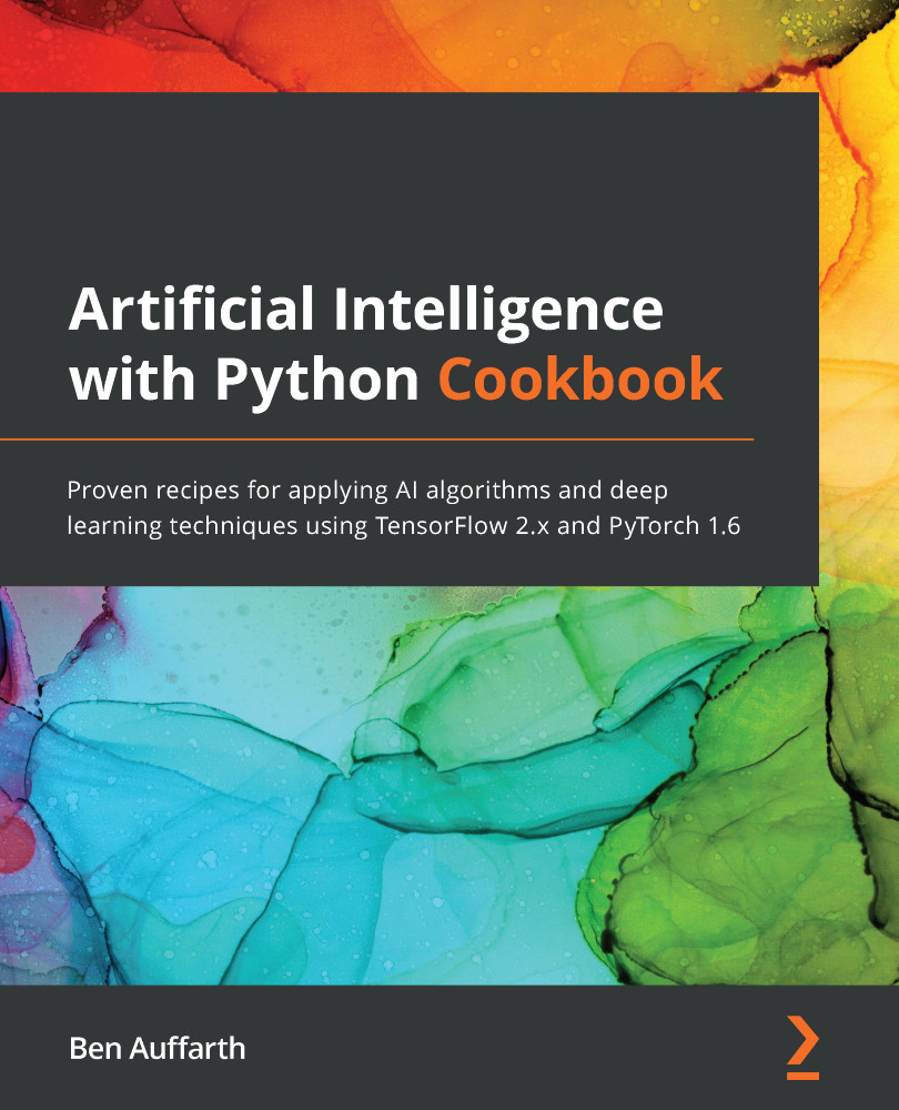
Artificial Intelligence with Python Cookbook
$45.99
Artificial Intelligence By Example
$45.99
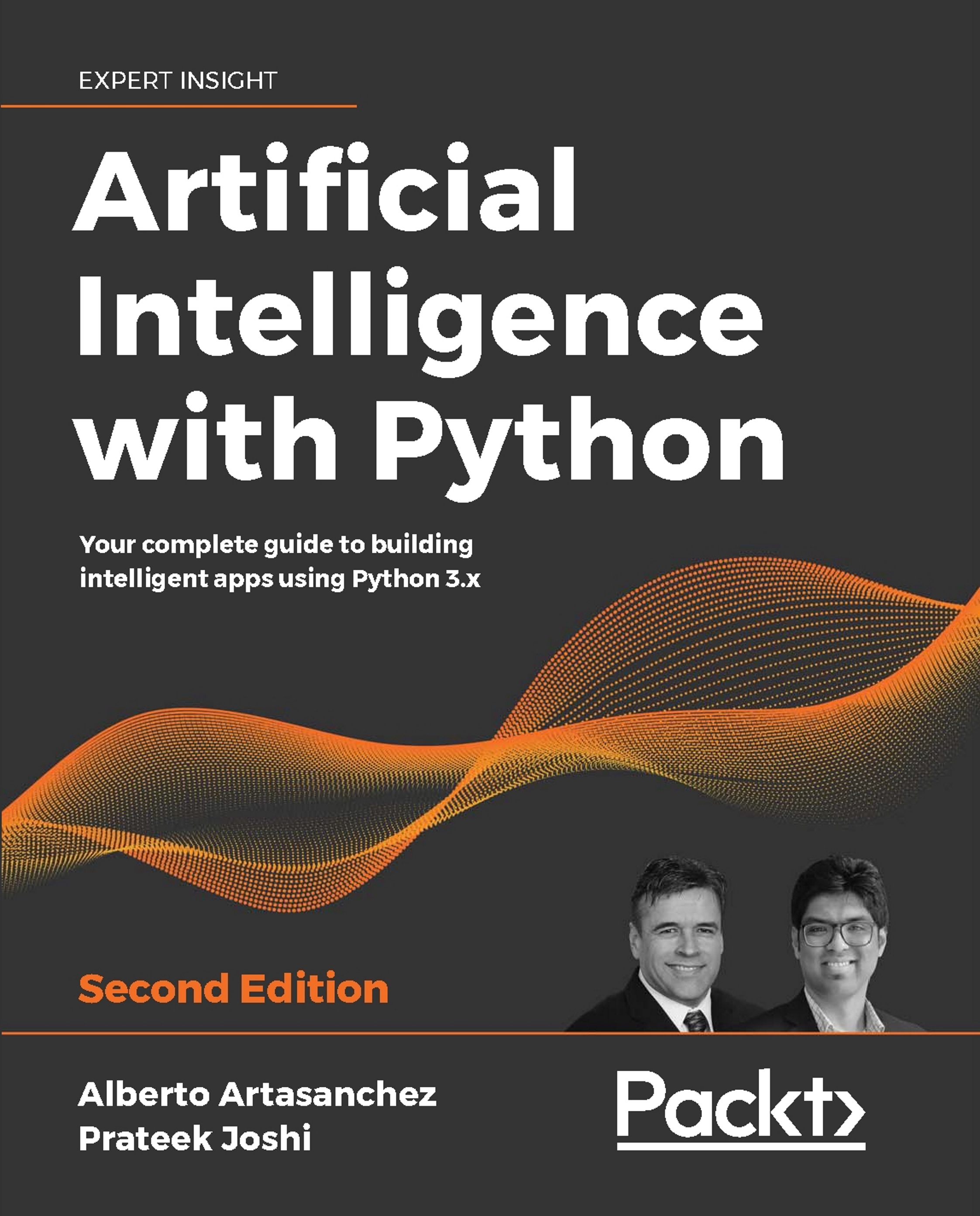
Artificial Intelligence with Python
$57.99
Total $ 149.97 Stars icon

Table of Contents

22 Chapters
Getting Started with Next-Generation Artificial Intelligence through Reinforcement Learning Chevron down icon Chevron up icon
Building a Reward Matrix – Designing Your Datasets Chevron down icon Chevron up icon
Machine Intelligence – Evaluation Functions and Numerical Convergence Chevron down icon Chevron up icon
Optimizing Your Solutions with K-Means Clustering Chevron down icon Chevron up icon
How to Use Decision Trees to Enhance K-Means Clustering Chevron down icon Chevron up icon
Innovating AI with Google Translate Chevron down icon Chevron up icon
Optimizing Blockchains with Naive Bayes Chevron down icon Chevron up icon
Solving the XOR Problem with a Feedforward Neural Network Chevron down icon Chevron up icon
Abstract Image Classification with Convolutional Neural Networks (CNNs) Chevron down icon Chevron up icon
Conceptual Representation Learning Chevron down icon Chevron up icon
Combining Reinforcement Learning and Deep Learning Chevron down icon Chevron up icon
AI and the Internet of Things (IoT) Chevron down icon Chevron up icon
Visualizing Networks with TensorFlow 2.x and TensorBoard Chevron down icon Chevron up icon
Preparing the Input of Chatbots with Restricted Boltzmann Machines (RBMs) and Principal Component Analysis (PCA) Chevron down icon Chevron up icon
Setting Up a Cognitive NLP UI/CUI Chatbot Chevron down icon Chevron up icon
Improving the Emotional Intelligence Deficiencies of Chatbots Chevron down icon Chevron up icon
Genetic Algorithms in Hybrid Neural Networks Chevron down icon Chevron up icon
Neuromorphic Computing Chevron down icon Chevron up icon
Quantum Computing Chevron down icon Chevron up icon
Answers to the Questions Chevron down icon Chevron up icon
Other Books You May Enjoy Chevron down icon Chevron up icon
Index Chevron down icon Chevron up icon

Customer reviews

Top Reviews
Rating distribution
Full star icon Full star icon Full star icon Full star icon Half star icon 4.6
(17 Ratings)
5 star 76.5%
4 star 11.8%
3 star 11.8%
2 star 0%
1 star 0%
Filter icon Filter
Top Reviews

Filter reviews by


Tamzid Bhuiyan May 19, 2021
Full star icon Full star icon Full star icon Full star icon Full star icon 5
information are helpful , good for students
Amazon Verified review Amazon
Jean-patrice Glafkides Mar 28, 2020
Full star icon Full star icon Full star icon Full star icon Full star icon 5
This is a big book that aim at showing all aspects of AI. It drives us trhu to almost all kind of AI as of now with sample. It helps me find quick information on some specific part of AI.
Amazon Verified review Amazon
Laura Mar 24, 2020
Full star icon Full star icon Full star icon Full star icon Full star icon 5
This book covers a breath of concepts not typically found in a single resource. Valuable for understanding both the theory and the applications of AI development. Very insightful!
Amazon Verified review Amazon
Pedro V. Marcal Mar 30, 2020
Full star icon Full star icon Full star icon Full star icon Full star icon 5
A long established mantra of AI is that 'data is program and program is data'. Nowhere is this more true than in Reinforcement Learning (RL) and Deep Learning (DL). Here there is no established theory, just established Algorithms. The author's book steps in and by careful building of examples illustrates the underlying principles behind RL and DL. Each example is explained by [1] explaining the basis of the required data. [2] a textual understanding of the problem. [3] the development of a Python based program to solve the problem.I recommend this book to those who wish to gain a better insight into RL and DL and are willing to work towards it.
Amazon Verified review Amazon
user Apr 03, 2020
Full star icon Full star icon Full star icon Full star icon Full star icon 5
There is only one way to learn data science: With a solid understanding of the underlying theory, and by getting your hands dirty with real examples, data, and code. AI by example delivers exactly this mix, with examples that go beyond contrived toy boxes, and real code on git.While I wish the book had a chapter how to assure ML by scrutinizing data, debugging models, assessing model competence, and how to apply general software engineering principles as algorithms are derived from data, I understand that these issues concern a more experienced audience and would be out of scope for beginners. Still, I can see this book as a reference even for more experienced professionals, and it would be great to see these aspects considered in a third edition.That said, this book is equally for developers who need to learn how to build solid machine learning programs, project managers and consultants need to learn what ML is and is not capable of, as well as teachers and students who get a comprehensive overview of the key aspects of AI, along with their first hands-on experience training models.
Amazon Verified review Amazon
Get free access to Packt library with over 7500+ books and video courses for 7 days!
Start Free Trial

FAQs

How do I buy and download an eBook? Chevron down icon Chevron up icon

Where there is an eBook version of a title available, you can buy it from the book details for that title. Add either the standalone eBook or the eBook and print book bundle to your shopping cart. Your eBook will show in your cart as a product on its own. After completing checkout and payment in the normal way, you will receive your receipt on the screen containing a link to a personalised PDF download file. This link will remain active for 30 days. You can download backup copies of the file by logging in to your account at any time.

If you already have Adobe reader installed, then clicking on the link will download and open the PDF file directly. If you don't, then save the PDF file on your machine and download the Reader to view it.

Please Note: Packt eBooks are non-returnable and non-refundable.

Packt eBook and Licensing When you buy an eBook from Packt Publishing, completing your purchase means you accept the terms of our licence agreement. Please read the full text of the agreement. In it we have tried to balance the need for the ebook to be usable for you the reader with our needs to protect the rights of us as Publishers and of our authors. In summary, the agreement says:

  • You may make copies of your eBook for your own use onto any machine
  • You may not pass copies of the eBook on to anyone else
How can I make a purchase on your website? Chevron down icon Chevron up icon

If you want to purchase a video course, eBook or Bundle (Print+eBook) please follow below steps:

  1. Register on our website using your email address and the password.
  2. Search for the title by name or ISBN using the search option.
  3. Select the title you want to purchase.
  4. Choose the format you wish to purchase the title in; if you order the Print Book, you get a free eBook copy of the same title. 
  5. Proceed with the checkout process (payment to be made using Credit Card, Debit Cart, or PayPal)
Where can I access support around an eBook? Chevron down icon Chevron up icon
  • If you experience a problem with using or installing Adobe Reader, the contact Adobe directly.
  • To view the errata for the book, see www.packtpub.com/support and view the pages for the title you have.
  • To view your account details or to download a new copy of the book go to www.packtpub.com/account
  • To contact us directly if a problem is not resolved, use www.packtpub.com/contact-us
What eBook formats do Packt support? Chevron down icon Chevron up icon

Our eBooks are currently available in a variety of formats such as PDF and ePubs. In the future, this may well change with trends and development in technology, but please note that our PDFs are not Adobe eBook Reader format, which has greater restrictions on security.

You will need to use Adobe Reader v9 or later in order to read Packt's PDF eBooks.

What are the benefits of eBooks? Chevron down icon Chevron up icon
  • You can get the information you need immediately
  • You can easily take them with you on a laptop
  • You can download them an unlimited number of times
  • You can print them out
  • They are copy-paste enabled
  • They are searchable
  • There is no password protection
  • They are lower price than print
  • They save resources and space
What is an eBook? Chevron down icon Chevron up icon

Packt eBooks are a complete electronic version of the print edition, available in PDF and ePub formats. Every piece of content down to the page numbering is the same. Because we save the costs of printing and shipping the book to you, we are able to offer eBooks at a lower cost than print editions.

When you have purchased an eBook, simply login to your account and click on the link in Your Download Area. We recommend you saving the file to your hard drive before opening it.

For optimal viewing of our eBooks, we recommend you download and install the free Adobe Reader version 9.

Modal Close icon
Modal Close icon