


In this chapter, we will cover the basic tasks of reading, storing, and cleaning data using Python and OpenRefine. You will learn the following recipes:
Reading and writing CSV/TSV files with Python
Reading and writing JSON files with Python
Reading and writing Excel files with Python
Reading and writing XML files with Python
Retrieving HTML pages with pandas
Storing and retrieving from a relational database
Storing and retrieving from MongoDB
Opening and transforming data with OpenRefine
Exploring the data with OpenRefine
Removing duplicates
Using regular expressions and GREL to clean up the data
Imputing missing observations
Normalizing and standardizing features
Binning the observations
Encoding categorical variables
For the following set of recipes, we will use Python to read data in various formats and store it in RDBMS and NoSQL databases.
All the source codes and datasets that we will use in this book are available in the GitHub repository for this book. To clone the repository, open your terminal of choice (on Windows, you can use command line, Cygwin, or Git Bash and in the Linux/Mac environment, you can go to Terminal) and issue the following command (in one line):
git clone https://github.com/drabastomek/practicalDataAnalysisCookbook.git
Tip
Note that you need Git installed on your machine. Refer to https://git-scm.com/book/en/v2/Getting-Started-Installing-Git for installation instructions.
In the following four sections, we will use a dataset that consists of 985 real estate transactions. The real estate sales took place in the Sacramento area over a period of five consecutive days. We downloaded the data from https://support.spatialkey.com/spatialkey-sample-csv-data/—in specificity, http://samplecsvs.s3.amazonaws.com/Sacramentorealestatetransactions.csv. The data was then transformed into various formats that are stored in the Data/Chapter01 folder in the GitHub repository.
In addition, you will learn how to retrieve information from HTML files. For this purpose, we will use the Wikipedia list of airports starting with the letter A, https://en.wikipedia.org/wiki/List_of_airports_by_IATA_code:_A.
To clean our dataset, we will use OpenRefine; it is a powerful tool to read, clean, and transform data.
CSV and TSV formats are essentially text files formatted in a specific way: the former one separates data using a comma and the latter uses tab \t characters. Thanks to this, they are really portable and facilitate the ease of sharing data between various platforms.
To execute this recipe, you will need the pandas module installed. These modules are all available in the Anaconda distribution of Python and no further work is required if you already use this distribution. Otherwise, you will need to install pandas and make sure that it loads properly.
Note
You can download Anaconda from http://docs.continuum.io/anaconda/install. If you already have Python installed but do not have pandas, you can download the package from https://github.com/pydata/pandas/releases/tag/v0.17.1 and follow the instructions to install it appropriately for your operating system (http://pandas.pydata.org/pandas-docs/stable/install.html).
No other prerequisites are required.
The
pandas module is a library that provides high-performing, high-level data structures (such as DataFrame) and some basic analytics tools for Python.
Note
The DataFrame is an Excel table-like data structure where each column represents a feature of your dataset (for example, the height and weight of people) and each row holds the data (for example, 1,000 random people's heights and weights). See http://pandas.pydata.org/pandas-docs/stable/dsintro.html#dataframe.
The module provides methods that make it very easy to read data stored in a variety of formats. Here's a snippet of a code that reads the data from CSV and TSV formats, stores it in a pandas DataFrame structure, and then writes it back to the disk (the read_csv.py file):
import pandas as pd

# names of files to read from
r_filenameCSV = '../../Data/Chapter01/realEstate_trans.csv'
r_filenameTSV = '../../Data/Chapter01/realEstate_trans.tsv'

# names of files to write to
w_filenameCSV = '../../Data/Chapter01/realEstate_trans.csv'
w_filenameTSV = '../../Data/Chapter01/realEstate_trans.tsv'

# read the data
csv_read = pd.read_csv(r_filenameCSV)
tsv_read = pd.read_csv(r_filenameTSV, sep='\t')

# print the first 10 records
print(csv_read.head(10))
print(tsv_read.head(10))

# write to files
with open(w_filenameCSV,'w') as write_csv:
    write_csv.write(tsv_read.to_csv(sep=',', index=False))

with open(w_filenameTSV,'w') as write_tsv:
    write_tsv.write(csv_read.to_csv(sep='\t', index=False))
Now, open the command-line console (on Windows, you can use either command line or Cygwin and in the Linux/Mac environment, you go to Terminal) and execute the following command:
python read_csv.py
You shall see an output similar to the following (abbreviated):
Baths beds      city        latitude   longitude    price  \
0      1     2  SACRAMENTO  38.631913 -121.434879  59222
1      1     3  SACRAMENTO  38.478902 -121.431028  68212
2      1     2  SACRAMENTO  38.618305 -121.443839  68880
...
Tip
Downloading the example code
You can download the example code files for this book from your account at http://www.packtpub.com. If you purchased this book elsewhere, you can visit http://www.packtpub.com/support and register to have the files e-mailed directly to you.
You can download the code files by following these steps:
Log in or register to our website using your e-mail address and password.
Hover the mouse pointer on the SUPPORT tab at the top.
Click on Code Downloads & Errata.
Enter the name of the book in the Search box.
Select the book for which you're looking to download the code files.
Choose from the drop-down menu where you purchased this book from.
Click on Code Download.
Once the file is downloaded, please make sure that you unzip or extract the folder using the latest version of:
WinRAR / 7-Zip for Windows
Zipeg / iZip / UnRarX for Mac
7-Zip / PeaZip for Linux
First, we load pandas to get access to the DataFrame and all its methods that we will use to read and write the data. Note that we alias the pandas module using as and specifying the name, pd; we do this so that later in the code we do not need to write the full name of the package when we want to access DataFrame or the read_csv(...) method. We store the filenames (for the reading and writing) in r_filenameCSV(TSV) and w_filenameCSV(TSV) respectively.
To read the data, we use pandas' read_csv(...) method. The method is very universal and accepts a variety of input parameters. However, at a minimum, the only required parameter is either the filename of the file or a buffer that is, an opened file object. In order to read the realEstate_trans.tsv file, you might want to specify the sep='\t' parameter; by default, read_csv(...) will try to infer the separator but I do not like to leave it to chance and always specify the separator explicitly.
As the two files hold exactly the same data, you can check whether the files were read properly by printing out some records. This can be accomplished using the .head(<no_of_rows>) method invoked on the DataFrame object, where <no_of_rows> specifies how many rows to print out.
Storing the data in pandas' DataFrame object means that it really does not matter what format the data was initially in; once read, it can then be saved in any format supported by pandas. In the preceding example, we write the contents read from a CSV file to a file in a TSV format.
The with open(...) as ...: structure should always be used to open files for either reading or writing. The advantage of opening files in this way is that it closes the file properly once you are done with reading from or writing to even if, for some reason, an exception occurs during the process.
Note
An exception is a situation that the programmer did not expect to see when he or she wrote the program.
Consider, for example, that you have a file where each line contains only one number: you open the file and start reading from it. As each line of the file is treated as text when read, you need to transform the read text into an integer—a data structure that a computer understands (and treats) as a number, not a text.
All is fine if your data really contains only numbers. However, as you will learn later in this chapter, all data that we gather is dirty in some way, so if, for instance, any of the rows contains a letter instead of a number, the transformation will fail and Python will raise an exception.
The open(<filename>, 'w') command opens the file specified by <filename> to write (the w parameter). Also, you can open files in read mode by specifying 'r' instead. If you open a file in the 'r+' mode, Python will allow a bi-directional flow of data (read and write) so you will be able to append contents at the end of the file if needed. You can also specify rb or wb for binary type of data (not text).
The .to_csv(...) method converts the content of a DataFrame to a format ready to store in a text file. You need to specify the separator, for example, sep=',', and whether the DataFrame index is to be stored in the file as well; by default, the index is also stored. As we do not want that, you should specify index=False.
Note
The DataFrame's index is essentially an easy way to identify, align, and access your data in the DataFrame. The index can be a consecutive list of numbers (just like row numbers in Excel) or dates; you can even specify two or more index columns. The index column is not part of your data (even though it is printed to screen when you print the DataFrame object). You can read more about indexing at http://pandas.pydata.org/pandas-docs/stable/indexing.html.
Described here is the easiest and quickest way of reading data from and writing data to CSV and TSV files. If you prefer to hold your data in a data structure other than pandas' DataFrame, you can use the csv module. You then read the data as follows (the read_csv_alternative.py file):
import csv

# names of files to read from
r_filenameCSV = '../../Data/Chapter01/realEstate_trans.csv'
r_filenameTSV = '../../Data/Chapter01/realEstate_trans.tsv'

# data structures to hold the data
csv_labels = []
tsv_labels = []
csv_data = []
tsv_data = []

# read the data
with open(r_filenameCSV, 'r') as csv_in:
    csv_reader = csv.reader(csv_in)

    # read the first line that holds column labels
    csv_labels = csv_reader.__next__()

    # iterate through all the records
    for record in csv_reader:
        csv_data.append(record)

with open(r_filenameTSV, 'r') as tsv_in:
    tsv_reader = csv.reader(tsv_in, delimiter='\t')

    tsv_labels = tsv_reader.__next__()

    for record in tsv_reader:
        tsv_data.append(record)

# print the labels
print(csv_labels, '\n')
print(tsv_labels, '\n')

# print the first 10 records
print(csv_data[0:10],'\n')
print(tsv_data[0:10],'\n')
We store the labels and data in separate lists, csv(tsv)_labels and csv(tsv)_data respectively. The .reader(...) method reads the data from the specified file line by line. To create a .reader(...) object, you need to pass an open CSV or TSV file object. In addition, if you want to read a TSV file, you need to specify the delimiter as well, just like DataFrame.
Tip
The csv module also provides the csv.writer object that allows saving data in a CSV/TSV format. See the documentation of the csv module at https://docs.python.org/3/library/csv.html.
Check the pandas documentation for read_csv(...) and write_csv(...) to learn more about the plethora of parameters these methods accept. The documentation can be found at http://pandas.pydata.org/pandas-docs/stable/io.html#io-read-csv-table.
JSON stands for JavaScript Object Notation. It is a hierarchical dictionary-like structure that stores key-value pairs separated by a comma; the key-value pairs are separated by a colon ':'. JSON is platform-independent (like XML, which we will cover in the Reading and writing XML files with Python recipe) making sharing data between platforms very easy. You can read more about JSON at http://www.w3schools.com/json/.
To execute this recipe, you will need Python with the pandas module installed. No other prerequisites are required.
The code to read a JSON file is as follows. Note that we assume the pandas module is already imported and aliased as pd (the read_json.py file):
# name of the JSON file to read from
r_filenameJSON = '../../Data/Chapter01/realEstate_trans.json'

# read the data
json_read = pd.read_json(r_filenameJSON)

# print the first 10 records
print(json_read.head(10))
This code works in a similar way to the one introduced in the previous section. First, you need to specify the name of the JSON file—we store it in the r_filenameJSON string. Next, use the read_json(...) method of pandas, passing r_filenameJSON as the only parameter.
The read data is stored in the json_read DataFrame object. We then print the bottom 10 observations using the .tail(...) method. To write a JSON file, you can use the .to_json() method on DataFrame and write the returned data to a file in a similar manner as discussed in the Reading and writing CSV/TSV files with Python recipe.
You can read and write JSON files using the json module as well. To read data from a JSON file, you can refer to the following code (the read_json_alternative.py file):
# read the data
with open('../../Data/Chapter01/realEstate_trans.json', 'r') \
    as json_file:
        json_read = json.loads(json_file.read())
This code reads the data from the realEstate_trans.json file and stores it in a json_read list. It uses the .read() method on a file that reads the whole content of the specified file into memory. To store the data in a JSON file, you can use the following code:
# write back to the file
with open('../../Data/Chapter01/realEstate_trans.json', 'w') \
    as json_file:
json_file.write(json.dumps(json_read))Check the pandas documentation for read_json at http://pandas.pydata.org/pandas-docs/stable/io.html#io-json-reader.
Microsoft Excel files are arguably the most widely used format to exchange data in a tabular form. In the newest incarnation of the XLSX format, Excel can store over one million rows and over 16 thousand columns in a single worksheet.
To execute this recipe, you will need the pandas module installed. No other prerequisites are required.
The following is the code to read the Excel file. Note that we assume the pandas module is already imported and aliased as pd (the read_xlsx.py file):
# name of files to read from and write to
r_filenameXLSX = '../../Data/Chapter01/realEstate_trans.xlsx'
w_filenameXLSX = '../../Data/Chapter01/realEstate_trans.xlsx'

# open the Excel file
xlsx_file = pd.ExcelFile(r_filenameXLSX)

# read the contents
xlsx_read = {
    sheetName: xlsx_file.parse(sheetName)
        for sheetName in xlsx_file.sheet_names
}

# print the first 10 prices for Sacramento
print(xlsx_read['Sacramento'].head(10)['price'])

# write to Excel
xlsx_read['Sacramento'] \
.to_excel(w_filenameXLSX, 'Sacramento', index=False)We follow a similar manner to the previous examples. We first open the XLSX file and assign it to the xlsx_file object using pandas' ExcelFile(...) method. We employ the .parse(...) method to do the work for us and read the contents of the specified worksheet; we store it in the xlsx_read dictionary. Note that you get access to all the worksheets in the Excel file through the .sheet_names property of the ExcelFile object.
To create the xlsx_read dictionary, we use Pythonic dictionary comprehension: instead of looping through the sheets explicitly and then adding the elements to the dictionary, we use the dictionary comprehension to make the code more readable and compact.
Note
The comprehensions make it easy to understand the code as they mimic mathematical notations. Consider, for example, the following list of powers of 2: (A = (20, 21, 22, ..., 28) = (2x: 0 <= x < 9), x is an integer). It can then easily be translated into Python using a list comprehension: A = [2**x for x in range(0, 9)]. This would create the following list: A = [1, 2, 4, 8, 16, 32, 64, 128, 256].
Also, in Python, the comprehensions are also a tiny bit faster than explicit loops (http://stackoverflow.com/questions/22108488/are-list-comprehensions-and-functional-functions-faster-than-for-loops).
The range(<from>,<to>) command generates a sequence of integers starting at <from> and extending to <to> less one. For example, range(0,3) will generate a sequence 0, 1, 2.
Storing the data in an Excel file is also very easy. All that is required is to invoke the .to_excel(...) method, where the first parameter is the name of the file you want to save the data to and the second one specifies the name of the worksheet. In our example, we also specified the additional index=False parameter that instructs the method not to save the index; by default, the .to_excel(...) method saves the index in column A.
Alternatively to reading Excel files using pandas' read_excel(...), there are multiple Python modules you can use that provide Excel data reading capabilities. pandas uses the xlrd (https://secure.simplistix.co.uk/svn/xlrd/trunk/xlrd/doc/xlrd.html?p=4966) module to read the data and then converts it to a DataFrame. For XLSX files, you can also use the openpyxl module (the read_xlsx_alternative.py file):
import openpyxl as oxl

# name of files to read from
r_filenameXLSX = '../../Data/Chapter01/realEstate_trans.xlsx'

# open the Excel file
xlsx_wb = oxl.load_workbook(filename=r_filenameXLSX)

# names of all the sheets in the workbook
sheets = xlsx_wb.get_sheet_names()

# extract the 'Sacramento' worksheet
xlsx_ws = xlsx_wb[sheets[0]]
We first read the contents of the Excel file and store it in xlsx_wb (workbook). From the workbook, we extract the names of all the worksheets and put it in the sheets variable. As we have only one worksheet in our workbook, the
sheets variable equals to 'Sacramento'. We use it to create an xlsx_ws object that allows iterating through all the rows:
labels = [cell.value for cell in xlsx_ws.rows[0]]

data = [] # list to hold the data

for row in xlsx_ws.rows[1:]:
    data.append([cell.value for cell in row])
The first row contains the labels for all the columns so it is a good idea to store this separately—we put it in the labels variable. We then iterate through all the rows in the worksheet, using the .rows iterator, and append the values of all the cells to the data list:
print(
    [item[labels.index('price')] for item in data[0:10]]
)
The last part of the code prints out the prices of properties for the top 10 rows. We use list comprehension to create a list of the prices. You can find the first occurrence of a certain item in a list by calling .index(...) on a list object, as we did in this example.
Check the pandas documentation for read_excel at http://pandas.pydata.org/pandas-docs/stable/io.html#io-excel. Also, you can visit http://www.python-excel.org for a list of modules that allow you to work with data stored in different Excel formats, both older .xls and newer .xlsx files.
XML stands for eXtensible Markup Language. Although not as popular to store data as the formats described previously, certain web APIs return XML-encoded information on request.
An XML-encoded document has a tree-like structure. To read the contents, we start at the root of the tree (normally, the name of the element that follows the XML declaration <?xml version="1.0" encoding="UTF-8"?>; every XML-encoded document needs to begin with such declaration). In our case, the root of our XML-encoded document is <records>. A single <record>...</record> contains a list of <var var_name=...>...</var>.
Note
Warning: The xml module is not secure. Caution is required when dealing with XML-encoded messages from untrusted sources. An attacker might access local files, carry out DoS attacks, and more. Refer to the documentation for the xml module at https://docs.python.org/3/library/xml.html.
In order to execute the following recipe, you need the pandas and xml modules available. No other prerequisites are required.
Reading the data from an XML file directly to a pandas DataFrame requires some supplementary code; this is because each XML file has a different structure and requires a made-to-fit parsing. We will define the innards of the methods defined in the following section of this recipe. The source code for this section can be found in the read_xml.py file:
import pandas as pd
import xml.etree.ElementTree as ET

def read_xml(xml_tree):
    '''
        Read an XML encoded data and return pd.DataFrame
    '''

def iter_records(records):
    '''
        Generator to iterate through all the records
    '''

def write_xml(xmlFileName, data):
    '''
        Save the data in an XML format
    '''

def xml_encode(row):
    '''
        Encode the row as an XML with a specific hierarchy
    '''

# names of files to read from and write to
r_filenameXML = '../../Data/Chapter01/realEstate_trans.xml'
w_filenameXML = '../../Data/Chapter01/realEstate_trans.xml'

# read the data
xml_read = read_xml(r_filenameXML)

# print the first 10 records
print(xml_read.head(10))

# write back to the file in an XML format
write_xml(w_filenameXML, xml_read)Let's analyze the preceding code step by step. First, we import all the modules that we need. The xml.etree.ElementTree module is a lightweight XML parser of the XML tree and we will use it to parse the XML structure of our file. As before, we define names of the files to read and write in separate variables (r_filenameXML, w_filenameXML).
To read the data from the XML-encoded file, we use the
read_xml(...) method:
def read_xml(xmlFileName):
    with open(xmlFileName, 'r') as xml_file:
        # read the data and store it as a tree
        tree = ET.parse(xml_file)

        # get the root of the tree
        root = tree.getroot()

        # return the DataFrame
        return pd.DataFrame(list(iter_records(root)))
The method takes the name of the file as its only parameter. First, the file is opened. Using the .parse(...) method, we create a tree-like structure from our XML-encoded file and store it in the tree object. We then extract the root using the .getroot() method on the tree object: this is the starting point to process the data further. The return statement calls the iter_records method passing the reference to the root of the tree and then converts the returned information to a DataFrame:
def iter_records(records):
    for record in records:
        # temporary dictionary to hold values
        temp_dict = {}

        # iterate through all the fields
        for var in record:
           temp_dict[
               var.attrib['var_name']
           ] = var.text

        # generate the value
        yield temp_dict
The iter_records method is a generator: a method that, as the name suggests, generates the values. Unlike regular methods that have to return all the values when the function finishes (a return statement), generators hand over the data back to the calling method one at a time (hence the yield keyword) until done.
Tip
For a more in-depth discussion on generators, I suggest reading https://www.jeffknupp.com/blog/2013/04/07/improve-your-python-yield-and-generators-explained/.
Our iter_records method, for each record read, emits a temp_dict dictionary object back to the read_xml method. Each element of the dictionary has a key equal to the var_name attribute of the <var> XML element. (Our <var> has the following format: <var var_name=...>.)
Tip
The <var> tag could have more attributes with other names—these would be stored in the .attrib dictionary (a property of the XML tree node) and would be accessible by their names—see the highlighted line in the previous source code.
The value of <var> (contained within <var>...</var>) is accessible through the .text property of the XML node, while the .tag property stores its name (in our case, var).
The return statement of the read_xml method creates a list from all the dictionaries passed, which is then turned into a DataFrame.
To write the data in an XML format, we use the write_xml(...) method:
def write_xml(xmlFileName, data):
    with open(xmlFileName, 'w') as xmlFile:

        # write the headers
        xmlFile.write(
            '<?xml version="1.0" encoding="UTF-8"?>\n'
        )
        xmlFile.write('<records>\n')

        # write the data
        xmlFile.write(
            '\n'.join(data.apply(xml_encode, axis=1))
        )

        # write the footer
        xmlFile.write('\n</records>')
The method opens the file specified by the xmlFileName parameter. Every XML file needs to start with the XML declaration (see the introduction to this recipe) in the first line. Then, we write out the root of our XML schema, <records>.
Next, it is time to write out the data. We use the .apply(...) method of the DataFrame object to iterate through the records contained within. Its first parameter specifies the method to be applied to each record. By default, the axis parameter is set to 0. This means that the method specified in the first parameter would be applied to each column of the DataFrame. By setting the parameter to 1, we instruct the .apply(...) method that we want to apply the xml_encode(...) method specified in the first parameter to each row. We use the
xml_encode(...) method to process each record from the data DataFrame:
def xml_encode(row):
    # first -- we output a record
    xmlItem = ['  <record>']

    # next -- for each field in the row we create a XML markup
    #         in a <field name=...>...</field> format
    for field in row.index:
        xmlItem \
            .append(
                '    <var var_name="{0}">{1}</var>' \
                .format(field, row[field])
            )

    # last -- this marks the end of the record
    xmlItem.append('  </record>')

    # return a string back to the calling method
    return '\n'.join(xmlItem)
The code creates a list of strings, xmlItem. The first element of the list is the <record> indicator and the last one will be </record>. Then, for each field in the row, we append values of each column for that record encapsulated within <var var_name=<column_name>><value></var>. The variables in bold indicate specific column names from the record (<column_name>) and corresponding value (<value>). Once all the fields of the record have been parsed, we create a long string by concatenating all the items of the xmlItem list using the '\n'.join(...) method. Each <var>...</var> tag is then separated by \n. The string is returned to the caller (write_xml). Each record is further concatenated in the write_xml(...) method and then output to the file. We finish with the closing tag, </records>.
Although not as popular to store large datasets as previous formats, sometimes we find data in a table on a web page. These structures are normally enclosed within the <table> </table> HTML tags. This recipe will show you how to retrieve data from a web page.
In order to execute the following recipe, you need pandas and re modules available. The re module is a regular expressions module for Python and we will use it to clean up the column names. Also, the read_html(...) method of pandas requires html5lib to be present on your computer. If you use the Anaconda distribution of Python, you can do it by issuing the following command from your command line:
conda install html5lib
Otherwise, you can download the source from https://github.com/html5lib/html5lib-python, unzip it, and install the module manually:
cd html5lib-python-parser
python setup.py install
No other prerequisites are required.
pandas makes it very easy to access, retrieve, and parse HTML files. All this can be done in two lines. The retrieve_html.py file contains more code than that and we will discuss it in the next section:
# url to retrieve
url = 'https://en.wikipedia.org/wiki/' + \
      'List_of_airports_by_IATA_code:_A'

# extract the data from the HTML
url_read = pd.read_html(url, header = 0)[0]The read_html(...) method of pandas parses the DOM of the HTML file and retrieves the data from all the tables. It accepts a URL, file, or raw string with HTML tags as the first parameter. In our example, we also specified header = 0 to extract the header from the table. The read_html(...) method returns a list of DataFrame objects, one for each table in the HTML file. The list of airports page from Wikipedia contains only one table so we only retrieve the first element from the returned list of DataFrames. That's it! The list of airports is already in the url_read object.
However, there are two issues with the data retrieved: column names contain whitespaces and separator rows are in the data. As the names can contain all variety of whitespace characters (space, tabulator, and so on), we use the re module:
import re

# regular expression to find any white spaces in a string
space = re.compile(r'\s+')

def fix_string_spaces(columnsToFix):
    '''
        Converts the spaces in the column name to underscore
    '''
    tempColumnNames = [] # list to hold fixed column names

    # loop through all the columns
    for item in columnsToFix:
        # if space is found
        if space.search(item):
            # fix and append to the list
            tempColumnNames \
                .append('_'.join(space.split(item)))
        else:
            # else append the original column name
            tempColumnNames.append(item)

    return tempColumnNames
First, we compile the regular expression that attempts to find at least one space in a word.
Tip
It goes beyond the scope of this book to discuss regular expressions in detail. A good compendium of knowledge on this topic can be found at https://www.packtpub.com/application-development/mastering-python-regular-expressions or in the re module documentation found at https://docs.python.org/3/library/re.html.
The method then loops through all the columns and, if it finds a space in the (space.search(...)) name, it then splits the column name (space.split(...)) into a list. The list is then concatenated using '_' as a separator. If, however, the column name contains no spaces, the original name is appended to the list of column names. To alter the column names in the DataFrame, we use the following code:
url_read.columns = fix_string_spaces(url_read.columns)
If you look at Wikipedia's list of airports table, you can see that it contains separator rows to group IATA names according to the first two letters of the code. All the other columns in the tables are missing. To deal with this issue, we can use DataFrame's .dropna(...) method.
Note
pandas has a couple of methods to deal with NaN (Not a Number) observations. In the Imputing missing observations recipe, we introduce the .fillna(...) method.
The .dropna(...) method drops rows (or columns if we want to) that contain at least one missing observation. However tempting it may be to just use .dropna(...) without any parameters, you would also drop all the legit rows that miss the Daylight Saving Time (DST) or ICAO code. We can, however, specify a threshold. A very rough look at the data leads to a conclusion that some legit records can contain up to two missing variables. The inplace=True parameter removes the data from the original DataFrame instead of creating a copy of the original one and returning a trimmed DataFrame; the default is inplace=False:
url_read.dropna(thresh=2, inplace=True)
Once we remove some rows, the DataFrame index will have holes. We can recreate it using the following code:
url_read.index = range(0,len(url_read))
To print out the top 10 IATA codes with corresponding airport names, we can use the following code:
print(url_read.head(10)[['IATA', 'Airport_name']])
If you want to retrieve more than one column, you put that in the form of a list; in our case, this was ['IATA', 'Airport_name']. The same results can be attained with the following code:
print(url_read[0:10][['IATA', 'Airport_name']])
The relational database model was invented in 1970 at IBM. Since then, it reigned the field of data analytics and storage for decades. The model is still widely used but has been losing the field to more and more popular solutions such as Hadoop. Nevertheless, the demise of relational databases is nowhere near as it is still a tool of choice for many applications.
In order to execute the following recipe, you need pandas and SQLAlchemy modules installed. The SQLAlchemy is a module that abstracts the database interactions between Python scripts and a number of relational databases; effectively, you do not have to remember the specifics of each database's syntax as SQLAlchemy will handle that for you.
If you are using the Anaconda distribution, issue the following command:
conda install sqlalchemy
Refer to your distribution of Python to check how to install new modules. Alternatively, check the previous recipe for instructions on how to install modules manually.
In addition, you might need to install the psycopg2 module. This can be accomplished with the following command:
conda install psycopg2
If, however, you are not using Anaconda, the psycopg2 can be found at http://initd.org/psycopg/. Follow the installation instructions found on the website.
To execute the script in this recipe, you will also need a PostgreSQL database running locally. Go to http://www.postgresql.org/download/ and follow the installation instructions for your operating system contained therein. We assume that you have your PostgreSQL database installed up and running before you proceed. We also assume that your database can be accessed at localhost:5432. On a Unix-like system, you can check the port used by the PostgreSQL database by issuing the following command in the terminal:
cat /etc/services | grep postgre
No other prerequisites are required.
pandas works hand in hand with SQLAlchemy to make accessing and storing/retrieving data in/from many databases very easy. Reading the data and storing it in the database can be achieved with the following script (the store_postgresql.py file):
import pandas as pd
import sqlalchemy as sa

# name of the CSV file to read from
r_filenameCSV = '../../Data/Chapter01/realEstate_trans.csv'

# database credentials
usr  = 'drabast'
pswd = 'pAck7!B0ok'

# create the connection to the database
engine = sa.create_engine(
    'postgresql://{0}:{1}@localhost:5432/{0}' \
    .format(usr, pswd)
)

# read the data
csv_read = pd.read_csv(r_filenameCSV)

# transform sale_date to a datetime object
csv_read['sale_date'] = pd.to_datetime(csv_read['sale_date'])

# store the data in the database
csv_read.to_sql('real_estate', engine, if_exists='replace')First, we import all the necessary modules: pandas and SQLAlchemy. We also store the name of the CSV file we will be reading the data from in a variable, and we specify the credentials to be used to connect to our PostgreSQL database. Then, using SQLAchemy's create_engine(...) method, we create an object that allows us to access the PostgreSQL database. The connection string specific syntax can be broken down as follows:
sa.create_engine('postgresql://<user_name>:<password>@<server>:<port>/<database>')Here, <user_name> is the username allowed to log in to <database> using <password>. The user needs (at a minimum) CREATE, DROP, INSERT, and SELECT privileges for the specified database. The <server> tag can be expressed as an IP address of the server running the PostgreSQL database or (as in our case) the name of the server (localhost). The <port> specifies the server port the database listens on.
Next, we read in the data from a CSV file and convert the sale_date column to a datetime object so that we can store the data in a date format in the database. The read_csv(...) method normally tries to infer the proper format for the data read from a file but it can get really tricky with dates. Here, we explicitly specify the date format for the sale_date column.
The last line of the script stores the information in the database. The to_sql(...) method specifies the name of the table ('real_estate') and connector (engine) to be used. The last parameter passed instructs the method to replace the table if it already exists in the database.
You can check whether the data has loaded properly using the following command:
query = 'SELECT * FROM real_estate LIMIT 10'
top10 = pd.read_sql_query(query, engine)
print(top10)
We first specify a valid SQL query and then use the
read_sql_query(...) method to execute it.
The most popular database in the world is SQLite. SQLite databases can be found in phones, TV sets, cars, among others; it makes SQLite the most widespread database. SQLite is very lightweight and requires no server to run. It can either store the data on a disk or use the memory of your computer to temporarily keep the data. The latter can be used when speed is required but the data disappears as soon as your script finishes.
With SQLAlchemy, it is also extremely easy to talk to the SQLite database. The only change required in the preceding example is how we construct the engine (the store_SQLite.py file):
# name of the SQLite database
rw_filenameSQLite = '../../Data/Chapter01/realEstate_trans.db'

# create the connection to the database
engine = sa.create_engine(
    'sqlite:///{0}'.format(rw_filenameSQLite)
)
As you can see, as the SQLite databases are serverless, the only required parameter is where to store the database file itself.
Tip
If, instead of storing the database in the file, you would like to keep your data in the computer's memory, use sqlite:// as the connection string.
Note
Note the three slashes in the path; this is to help the innards of the create_engine(...) method. At the most general level, the connection string follows the following pattern:
<database_type>://<server_information>/<database>
As SQLite databases do not require any server, <server_information> is empty and, hence, three slashes.
I highly recommend checking out the documentation for SQLAlchemy as it is a very powerful middleman between your code and various databases; the documentation can be found at http://docs.sqlalchemy.org/en/rel_1_0/index.html.
MongoDB has become one of the most popular, so-called, NoSQL databases that are there. It is highly scalable, has a very flexible data model and highly expressive query language. MongoDB is highly popular for storing unstructured data, especially for web-based apps: MEAN.js combines MongoDB, Express.js, Angular.js, and Node.js in one fullstack framework.
You need to have pandas and PyMongo modules installed. If you do not have PyMongo, you can either use conda to install the missing package or go to http://api.mongodb.org/python/current/installation.html#installing-from-source and follow the steps listed there.
Also, you need the MongoDB database up and running on your computer. You can download MongoDB from https://www.mongodb.org/downloads and then follow the instructions listed at http://docs.mongodb.org/manual/installation/ for your operating system.
No other prerequisites are required.
Accessing and storing documents in MongoDB is almost effortless. We assume that the data to store in the database are accessible to us in a pandas' DataFrame object csv_read (the store_mongodb.py file):
# connect to the MongoDB database
client = pymongo.MongoClient()

# and select packt database
db = client['packt']

# then connect to real_estate collection
real_estate = db['real_estate']

# and then insert the data
real_estate.insert(csv_read.to_dict(orient='records'))
We first create a connection to MongoDB. As we are not passing any arguments to the MongoClient(...) method, PyMongo will connect to the default MongoDB database running on localhost and listening on port 27017. If you would like to connect to a different database, you can override these defaults; assuming that the database you want to connect to runs on a server with IP 10.92.1.12 and listens on a port 1234, you can use the following code:
client = pymongo.MongoClient(host='10.92.1.12', port=1234)
Tip
A full list of the MongoClient(...) method's available parameters with explanations is available at http://api.mongodb.org/python/current/api/pymongo/mongo_client.html.
The MongoClient(...) method automatically connects to the MongoDB database so there is no need to do it manually. Once connected, we connect to the internal database object we are after (in our case, we called it packt) and we store it in the db object. Depending on whether the real_estate collection exists or not in the database, the next line of our script either opens the collection or creates a new one, respectively. We then get access to this collection through the real_estate object.
Note
In MongoDB, collections are equivalents of tables. Each collection consists of documents, equivalents to records from the relational database world.
Then, and only then, we can start storing our documents in the collection. We use the insert(...) method to load the data to the collection.
Note
We use version 2.8 of PyMongo. In the newest (at the time of writing this book) stable version 3.0, the insert(...) method was deprecated in favor of insert_many(...). Refer to the documentation of your version of PyMongo at http://api.mongodb.org/python/2.8/api/index.html or http://api.mongodb.org/python/3.0/api/index.html.
The insert(...) method accepts a list of dictionaries. We use DataFrame's to_dict(...) method that does all the heavy lifting for us in transforming the data into a list of dictionaries. The orient='records' option instructs the method to return a list where each element is a dictionary with column names as keys and corresponding values. Each element of the resulting list will form a document in the collection.
The insert(...) method appends the data by default. If this is not desired, you can use the following code to remove all the documents from the collection before inserting into it:
# if there are any documents stored already -- remove them
if real_estate.count() > 0:
    real_estate.remove()
The count() method calculates the total number of documents in the collection—if there are any, the remove() method deletes all the documents.
Next, we want to print top 10 sales (by record ID) from ZIP codes 95841 and 95842. We can do it easily by querying our collection:
sales = real_estate.find({'zip': {'$in': [95841, 95842]}})
for sale in sales.sort('_id').limit(10):
    print(sale)
First, we extract all the sales from these ZIP codes. In our data, the field name we are after is zip. The $in operator works in the same way as the ANSI SQL expression IN (...) so we can specify a list of all the ZIP codes that we want to retrieve from the database. The find(...) method returns a cursor object; the cursor object is a generator. So, we use it to iterate through all the sales and print out each individual sale to the screen.
I suggest referring to the documentation of MongoDB at http://docs.mongodb.org/v2.6/ and
PyMongo for more details.
OpenRefine originated as GoogleRefine. Google later open sourced the code. It is a great tool to sift through the data quickly, clean it, remove duplicate rows, analyze distributions or trends over time, and more.
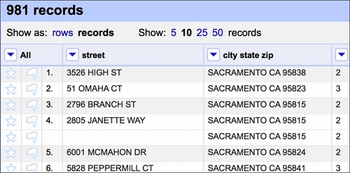
In this and the following recipes, we will deal with the realEstate_trans_dirty.csv file that is located in the Data/Chapter1 folder. The file has several issues that, over the course of the following recipes, we will see how to resolve.
First, when read from a text file, OpenRefine defaults the types of data to text; we will deal with data type transformations in this recipe. Otherwise, we will not be able to use facets to explore the numerical columns. Second, there are duplicates in the dataset (we will deal with them in the Remove duplicates recipe). Third, the city_state_zip column, as the name suggests, is an amalgam of city, state, and zip. We prefer keeping these separate, and in the Using regular expressions and GREL to clean up data recipe, we will see how to extract such information. There is also some missing information about the sale price—we will impute the sale prices in the Imputing missing observations recipe.
To run through these examples, you need OpenRefine installed and running on your computer. You can download OpenRefine from http://openrefine.org/download.html. The installation instructions can be found at https://github.com/OpenRefine/OpenRefine/wiki/Installation-Instructions.
OpenRefine runs in a browser so you need an Internet browser installed on your computer. I tested it in Chrome and Safari and found no issues.
Note
The Mac OS X Yosemite comes with Java 8 installed by default. OpenRefine does not support it. You need to install Java 6 or 7—see https://support.apple.com/kb/DL1572?locale=en_US.
However, even after installing legacy versions of Java, I still experienced some issues with version 2.5 of OpenRefine on Mac OS X Yosemite and El Capitan. Using the beta version (2.6), even though it is still in development, worked fine.
No other prerequisites are required.
First, you need to start OpenRefine, open your browser, and type http://localhost:3333. A window similar to the following screenshot should open:
The first thing you want to do is create a project. Click on Choose files, navigate to Data/Chapter1, and select realEstate_trans_dirty.csv. Click OK, then Next, and Create Project. After the data opens, you should see something similar to this:
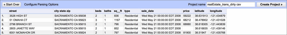
Note that the beds, baths, sq__ft, price, latitude, and longitude data is treated as text and so is sale_date. While converting the former is easy, the format of sale_date is not as easy to play with in OpenRefine:
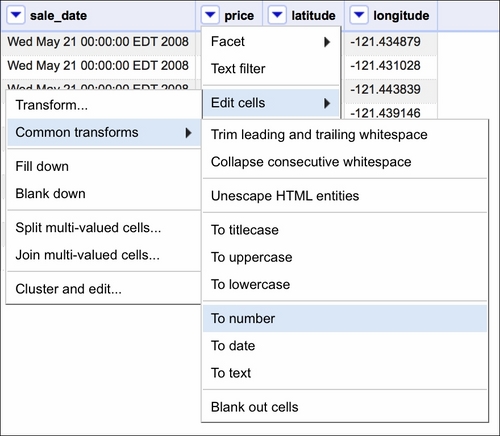
If the text data was in a format resembling, for example, 2008-05-21, we could just use the Google Refine Expression Language (GREL) method .toDate() and OpenRefine would convert the dates for us. In our case, we need to use some trickery to convert the dates properly. First, we select a Transform option, as shown in the following screenshot:
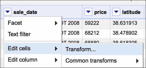
Then, in the window that opens, we will use GREL to convert the dates as follows:
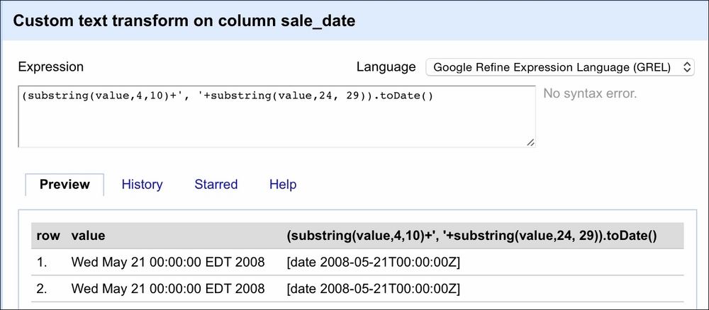
The value variable here represents the value of each cell in the selected column (sale_date). The first part of the expression extracts the month and day from the value, that is, we get in return May 21 by specifying that we want to retrieve a substring starting at the fourth character and finishing at the tenth character. The second substring(...) method extracts the year from the string. We separate the two by a comma using the ...+', '+... expression. The resulting value will result in the May 21, 2008 string pattern. Now OpenRefine can deal with this easily. Thus, we wrap our two substring methods inside parentheses and use the .toDate() method to convert the date properly. The Preview tab in the right column shows you the effect of our expression.
A very good introduction and deep dives into the various aspects of OpenRefine can be found in the Using OpenRefine book by Ruben Verborgh and Max De Wilde at https://www.packtpub.com/big-data-and-business-intelligence/using-openrefine.
Understanding your data is the first step to build successful models. Without intimate knowledge of your data, you might build a model that performs beautifully in the lab but fails gravely in production. Exploring the dataset is also a great way to see if there are any problems with the data contained within.
To follow this recipe, you need to have OpenRefine and virtually any Internet browser installed on your computer. See the Opening and transforming data with OpenRefine recipe's Getting ready subsection to see how to install OpenRefine.
We assume that you followed the previous recipe so your data is already loaded to OpenRefine and the data types are now representative of what the columns hold. No other prerequisites are required.
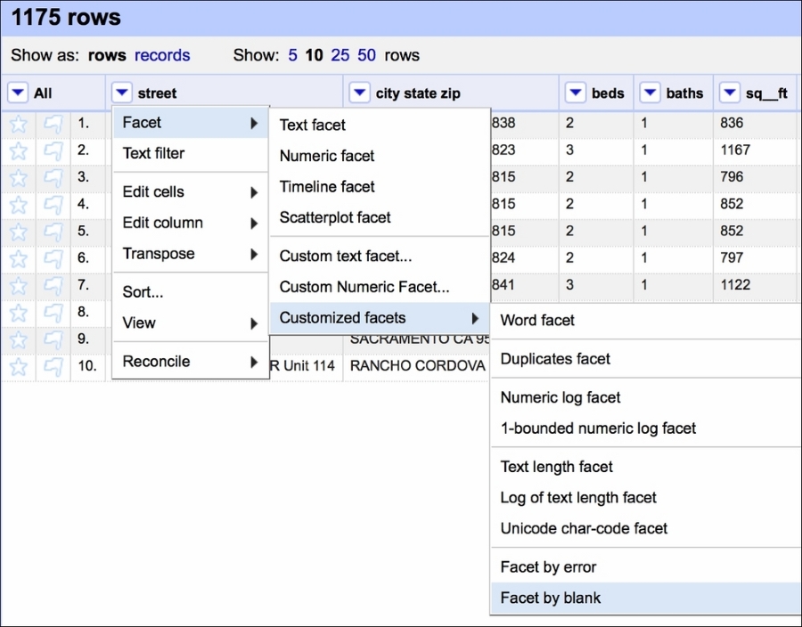
Exploring data in OpenRefine is easy with Facets. An OpenRefine Facet can be understood as a filter: it allows you to quickly either select certain rows or explore the data in a more straightforward way. A facet can be created for each column—just click on the down-pointing arrow next to the column and, from the menu, select the Facet group.
There are four basic types of facet in OpenRefine: text, numeric, timeline, and scatterplot.
Tip
You can create your own custom facets or also use some more sophisticated ones from the OpenRefine arsenal such as word or text lengths facets (among others).
The text facet allows you to get a sense of the distribution of text columns from your dataset quickly. For example, we can see which city in our dataset had the most sales between May 15, 2008 and May 21, 2008. As expected, since we analyze data from the Sacramento area, the city tops the list, followed by Elk Grove, Lincoln, and Roseville, as shown in the following screenshot:
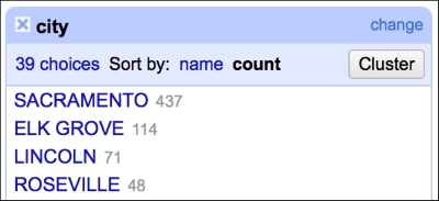
This gives you a very easy and straightforward insight on whether the data makes sense or not; you can readily determine whether the provided data is what it was supposed to be.
The numeric facet allows you to glimpse the distribution of your numeric data. We can, for instance, check the distribution of prices in our dataset, as shown in the following screenshot:
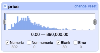
The distribution of the prices roughly follows what we would expect: left (positive) skewed distribution of sales prices makes sense, as one would expect less sales at the far right end of the spectrum, that is, people having money and willingness to purchase a 10-bedroom villa.
This facet reveals one of the flaws of our dataset: there are 89 missing observations in the price column. We will deal with these later in the book, in the Imputing missing observations recipe.
It is also good to check whether there are any blanks in the timeline of sales, as we were told that we would get seven days of data (May 15 to May 21, 2008):
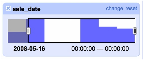
Our data indeed spans seven days but we see two days with no sales. A quick check of the calendar reveals that May 17 and May 18 was a weekend so there are no issues here. The timeline facet allows you to filter the data using the sliders on each side; here, we filtered observations from May 16, 2008 onward.
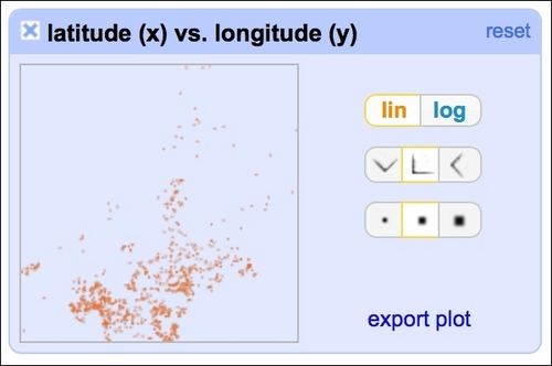
The scatterplot facet lets you analyze interactions between all the numerical variables in the dataset:
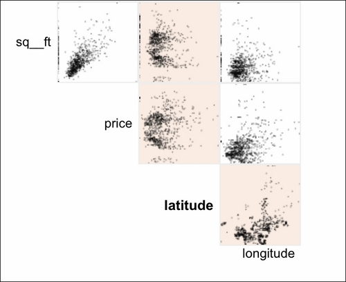
By clicking at the particular row and column, you can analyze the interactions in greater detail:
We can safely assume that all the data that lands on our desks is dirty (until proven otherwise). It is a good habit to check whether everything with our data is in order. The first thing I always check for is the duplication of rows.
To follow this recipe, you need to have OpenRefine and virtually any Internet browser installed on your computer.
We assume that you followed the previous recipes and your data is already loaded to OpenRefine and the data types are now representative of what the columns hold. No other prerequisites are required.
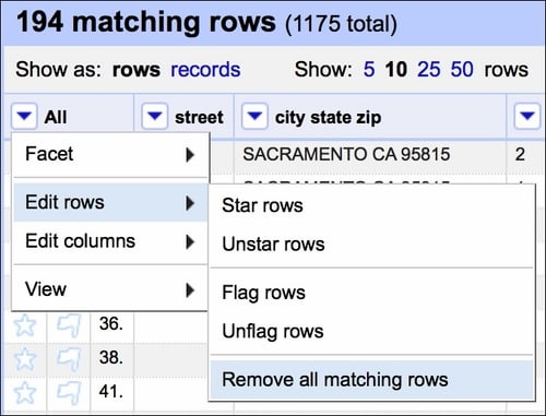
First, we assume that within the seven days of property sales, a row is a duplicate if the same address appears twice (or more) in the dataset. It is quite unlikely that the same house is sold twice (or more times) within such a short period of time. Therefore, first, we Blank down the observations if they repeat:
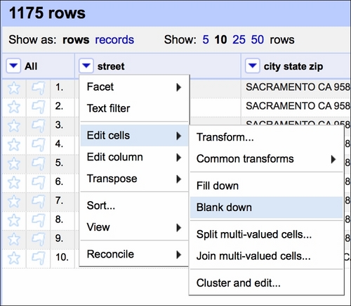
This effects in keeping only the first occurrence of a certain set of observations and blanking the rest (see the fourth row in the following screenshot):
Tip
The Fill down option has the opposite effect—it would fill in the blanks with the values from the row above unless the cell is not blank.
We can now create a Facet by blank that would allow us to quickly select the blanked rows:
Creating such a facet allows us to quickly select all the rows that are blank and remove them from the dataset:
Our dataset now has no duplicate records.
When cleaning up and preparing data for use, we sometimes need to extract some information from text fields. Occasionally, we can just split the text fields using delimiters. However, when a pattern of data does not allow us to simply split the text, we need to revert to regular expressions.
To follow this recipe, you need to have OpenRefine and virtually any Internet browser installed on your computer.
We assume that you followed the previous recipes and your data is already loaded to OpenRefine and the data types are now representative of what the columns hold. No other prerequisites are required.
First, let's have a look at the pattern that occurs in our city_state_zip column. As the name suggests, we can expect the first element to be the city followed by state and then a 5-digit ZIP code. We could just split the text field using a space character as a delimiter and be done with it. It would work for many records (for example, Sacramento) and they would be parsed properly into city, state, and ZIP. There is one problem with this approach—some locations consist of two or three words (for example, Elk Grove). Hence, we need a slightly different approach to extract such information.
This is where regular expressions play an invaluable role. You can use regular expressions in OpenRefine to transform the data. We will now split city_state_zip into three columns: city, state, and zip. Click on the downward button next to the name of the column and, from the menu, select Edit column and Add column based on this column. A window should appear, as shown in the following screenshot:
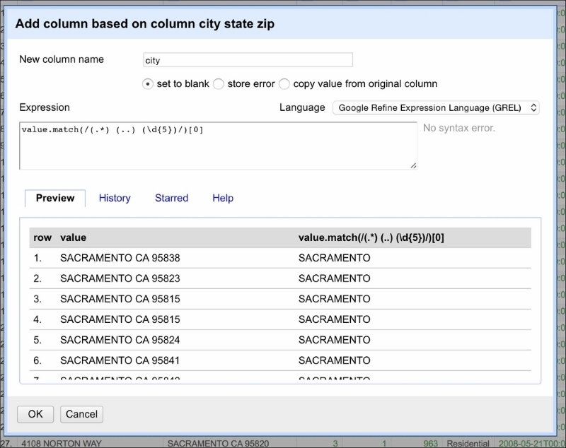
As before, the value represents the value of each cell. The .match(...) method is applied to the cell's value. It takes a regular expression as its parameter and returns a list of values matched given the expressed pattern. The regular expression is encapsulated between /.../. Let's break the regular expression down step by step.
We know the pattern of the city_state_zip column: first is the name of the city (can be more than one word), followed by a two-character state acronym, and ending with a 5-digit ZIP code. The regular expression to match such a pattern will be as follows:
(.*) (..) (\d{5})It is easier to read this expression starting from the end. So, reading from the right, first we extract the ZIP code using (\d{5}). The \d indicates any digit (and is equivalent to stating ([0-9]{5})) and {5} selects five digits from the back of the string. Next, we have (..)¬. This expression extracts the two-character acronym of the state identified by two dots (..). Note that we used ¬ in place of a space character just for readability purposes. This expression extracts only two characters and a space from the string—no less, no more. The last (reading from the right) is (.*) that can be understood as: extract all the characters (if any) that will not be matched by the other two expressions.
In entirety, the expression can be translated into English as follows: extract a string (even if empty) until a two-character acronym of the state is encountered (preceded by a space character) followed by a space and five digits indicating the ZIP code.
The .match(...) method generates a list. In our case, we will get back a list of three elements. To extract city, we select the first element from that list [0]. To select state and ZIP, we will repeat the same steps but select [1] and [2] respectively.
Now that we're done with splitting the city_state_zip column, we can export the project to a file. In the top right corner of the tool, you will find the Export button; select Comma-separated value. This will download the file automatically to your Downloads folder.
I highly recommend reading the Mastering Python Regular Expressions book by Felix Lopez and Victor Romero available at https://www.packtpub.com/application-development/mastering-python-regular-expressions.
Collecting data is messy. Research data collection instruments fail, humans do not want to answer some questions in a questionnaire, or files might get corrupted; these are but a sample of reasons why a dataset might have missing observations. If we want to use the dataset, we have a couple of choices: remove the missing observations altogether or replace them with some value.
To execute this recipe, you will need the pandas module.
No other prerequisites are required.
Once again, we assume that the reader followed the earlier recipes and the csv_read DataFrame is already accessible to us. To impute missing observations, all you need to do is add this snippet to your code (the data_imput.py file):
# impute mean in place of NaNs
csv_read['price_mean'] = csv_read['price'] \
    .fillna(
        csv_read.groupby('zip')['price'].transform('mean')
)The pandas' .fillna(...) method does all the heavy lifting for us. It is a DataFrame method that takes the value to be imputed as its only required parameter.
Tip
Consult the pandas documentation of .fillna(...) to see other parameters that can be passed to the method. The documentation can be found at http://pandas.pydata.org/pandas-docs/stable/generated/pandas.DataFrame.fillna.html.
In our approach, we assumed that each ZIP code might have different price averages. This is why we first grouped the observations using the .groupby(...) method. It stands to reason that the prices of houses would also heavily depend on the number of rooms in a given house; if our dataset had more observations, we would have added the beds variable as well.
The .groupby(...) method returns a GroupBy object. The .transform(...) method of the GroupBy object effectively replaces all the observations within ZIP code groups with a specified value, in our case, the mean for each ZIP code.
The .fillna(...) method now simply replaces the missing observations with the mean of the ZIP code.
Imputing the mean is not the only way to fill in the blanks. It returns a reasonable value only if the distribution of prices is symmetrical and without many outliers; if the distribution is skewed, the average is biased. A better metric of central tendency is the median. It takes one simple change in the way we presented earlier:
# impute median in place of NaNs
csv_read['price_median'] = csv_read['price'] \
    .fillna(
        csv_read.groupby('zip')['price'].transform('median')
)We normalize (or standardize) data for computational efficiency and so we do not exceed the computer's limits. It is also advised to do so if we want to explore relationships between variables in a model.
Tip
Computers have limits: there is an upper bound to how big an integer value can be (although, on 64-bit machines, this is, for now, no longer an issue) and how good a precision can be for floating-point values.
Normalization transforms all the observations so that all their values fall between 0 and 1 (inclusive). Standardization shifts the distribution so that the mean of the resultant values is 0 and standard deviation equals 1.
To execute this recipe, you will need the pandas module.
No other prerequisites are required.
To perform normalization and standardization, we define two helper functions (the data_standardize.py file):
def normalize(col):
    '''
        Normalize column
    '''
    return (col - col.min()) / (col.max() - col.min())

def standardize(col):
    '''
        Standardize column
    '''
return (col - col.mean()) / col.std()To normalize a set of observations, that is, to make each and every single one of them to be between 0 and 1, we subtract the minimum value from each observation and divide it by the range of the sample. The range in statistics is defined as a difference between the maximum and minimum value in the sample. Our normalize(...) method does exactly as described previously: it takes a set of values, subtracts the minimum from each observation, and divides it by the range.
Standardization works in a similar way: it subtracts the mean from each observation and divides the result by the standard deviation of the sample. This way, the resulting sample has a mean equal to 0 and standard deviation equal to 1. Our
standardize(...) method performs these steps for us:
csv_read['n_price_mean'] = normalize(csv_read['price_mean'])
csv_read['s_price_mean'] = standardize(csv_read['price_mean'])
Binning the observations comes in handy when we want to check the shape of the distribution visually or we want to transform the data into an ordinal form.
To execute this recipe, you will need the pandas and NumPy modules.
No other prerequisites are required.
To bin your observations (as in a histogram), you can use the following code (data_binning.py file):
# create bins for the price that are based on the
# linearly spaced range of the price values
bins = np.linspace(
    csv_read['price_mean'].min(),
    csv_read['price_mean'].max(),
    6
)

# and apply the bins to the data
csv_read['b_price'] = np.digitize(
    csv_read['price_mean'],
    bins
)First, we create bins. For our price (with the mean imputed in place of missing observations), we create six bins, evenly spread between the minimum and maximum values for the price. The .linspace(...) method does exactly this: it creates a NumPy array with six elements, each greater than the preceding one by the same value. For example, a .linspace(0,6,6) command would generate an array, [0., 1.2, 2.4, 3.6, 4.8, 6.].
Note
NumPy is a powerful numerical library for linear algebra. It can easily handle large arrays and matrices and offers a plethora of supplemental functions to operate on such data. For more information, visit http://www.numpy.org.
The .digitize(...) method returns, for each value in the specified column, the index of the bin that the value belongs to. The first parameter is the column to be binned and the second one is the array with bins.
To count the records within each bin, we use the .value_counts() method of DataFrame, counts_b = csv_read['b_price'].value_counts().
Sometimes, instead of having evenly-spaced values, we would like to have equal counts in each bucket. To attain such a goal, we can use quantiles.
Tip
Quantiles are closely related to percentiles. The difference is percentiles return values at a given sample percentage, while quantiles return values at the sample fraction. For more information, visit https://www.stat.auckland.ac.nz/~ihaka/787/lectures-quantiles-handouts.pdf.
What we want to achieve is splitting our column into deciles, that is, 10 bins of (more or less) equal size. To do this, we can use the following code (you can easily spot the similarities with the previous approach):
# create bins based on deciles
decile = csv_read['price_mean'].quantile(np.linspace(0,1,11))

# and apply the decile bins to the data
csv_read['p_price'] = np.digitize(
    csv_read['price_mean'],
    decile
)
The .quantile(...) method can either take one number (between 0 and 1) indicating the percentile to return (for example, 0.5 being the median and 0.25 and 0.75 being lower and upper quartiles). However, it can also return an array of values corresponding to the percentiles passed as a list to the method. The .linspace(0,1,11) command will produce the following array:
[ 0., 0.1, 0.2, 0.3, 0.4, 0.5, 0.6, 0.7, 0.8, 0.9, 1. ]
So, the .quantile(...) method will return a list starting with a minimum and followed by all the deciles up to the maximum for the price_mean column.
The final step on the road to prepare the data for the exploratory phase is to bin categorical variables. Some software packages do this behind the scenes, but it is good to understand when and how to do it.
Any statistical model can accept only numerical data. Categorical data (sometimes can be expressed as digits depending on the context) cannot be used in a model straightaway. To use them, we encode them, that is, give them a unique numerical code. This is to explain when. As for how—you can use the following recipe.
To execute this recipe, you will need the pandas module.
No other prerequisites are required.
Once again, pandas already has a method that does all of this for us (the data_dummy_code.py file):
# dummy code the column with the type of the property
csv_read = pd.get_dummies(
    csv_read,
    prefix='d',
    columns=['type']
)The .get_dummies(...) method converts categorical variables into dummy variables. For example, consider a variable with three different levels:
1  One
2  Two
3  Three
We will need three columns to code it:
1  One  1  0  0
2  Two  0   1  0
3  Three  0  0  1
Sometimes, we can get away with using only two additional columns. However, we can use this trick only if one of the levels is, effectively, null:
1  One  1  0
2  Two  0  1
3  Zero  0  0
The first parameter to the .get_dummies(...) method is the DataFrame. The columns parameter specifies the column (or columns, as we can also pass a list) in the DataFrame to the dummy code. Specifying the prefix, we instruct the method that the names of the new columns generated should have the d_ prefix; in our example, the generated dummy-coded columns will have d_Condo names (as an example). The underscore _ character is default but can also be altered by specifying the prefix_sep parameter.
Tip
For a full list of parameters to the .get_dummies(...) method, see http://pandas.pydata.org/pandas-docs/stable/generated/pandas.get_dummies.html.