Creating a multi-label classifier to label watches

A neural network is not limited to modeling the distribution of a single variable. In fact, it can easily handle instances where each image has multiple labels associated with it. In this recipe, we'll implement a CNN to classify the gender and style/usage of watches.

Let's get started.

Getting ready

First, we must install Pillow:

$> pip install Pillow

Next, we'll use the Fashion Product Images (Small) dataset hosted in Kaggle, which, after signing in, you can download here: https://www.kaggle.com/paramaggarwal/fashion-product-images-small. In this recipe, we assume the data is inside the ~/.keras/datasets directory, under the name fashion-product-images-small. We'll only use a subset of the data, focused on watches, which we'll construct programmatically in the How to do it… section.

Here are some sample images:

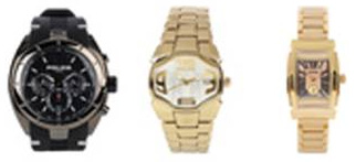
Figure 2.3 – Example images

Let's begin the recipe.

How to do it…

Let's review the steps to complete the recipe:

1. Import the necessary packages:

   import os
   import pathlib
   from csv import DictReader
   import glob
   import numpy as np
   from sklearn.model_selection import train_test_split
   from sklearn.preprocessing import MultiLabelBinarizer
   from tensorflow.keras.layers import *
   from tensorflow.keras.models import Model
   from tensorflow.keras.preprocessing.image import *

2. Define a function to build the network architecture. First, implement the convolutional blocks:

   def build_network(width, height, depth, classes):
       input_layer = Input(shape=(width, height, depth))
       x = Conv2D(filters=32,
                  kernel_size=(3, 3),
                  padding='same')(input_layer)
       x = ReLU()(x)
       x = BatchNormalization(axis=-1)(x)
       x = Conv2D(filters=32,
                  kernel_size=(3, 3),
                  padding='same')(x)
       x = ReLU()(x)
       x = BatchNormalization(axis=-1)(x)
       x = MaxPooling2D(pool_size=(2, 2))(x)
       x = Dropout(rate=0.25)(x)
       x = Conv2D(filters=64,
                  kernel_size=(3, 3),
                  padding='same')(x)
       x = ReLU()(x)
       x = BatchNormalization(axis=-1)(x)
       x = Conv2D(filters=64,
                  kernel_size=(3, 3),
                  padding='same')(x)
       x = ReLU()(x)
       x = BatchNormalization(axis=-1)(x)
       x = MaxPooling2D(pool_size=(2, 2))(x)
       x = Dropout(rate=0.25)(x)

   Next, add the fully convolutional layers:

       x = Flatten()(x)
       x = Dense(units=512)(x)
       x = ReLU()(x)
       x = BatchNormalization(axis=-1)(x)
       x = Dropout(rate=0.5)(x)
       x = Dense(units=classes)(x)
       output = Activation('sigmoid')(x)
       return Model(input_layer, output)

3. Define a function to load all images and labels (gender and usage), given a list of image paths and a dictionary of metadata associated with each of them:

   def load_images_and_labels(image_paths, styles, 
                              target_size):
       images = []
       labels = []
       for image_path in image_paths:
           image = load_img(image_path, 
                            target_size=target_size)
           image = img_to_array(image)
           image_id = image_path.split(os.path.sep)[-
                                            1][:-4]
           image_style = styles[image_id]
           label = (image_style['gender'], 
                    image_style['usage'])
           images.append(image)
           labels.append(label)
       return np.array(images), np.array(labels)

4. Set the random seed to guarantee reproducibility:

   SEED = 999
   np.random.seed(SEED)

5. Define the paths to the images and the styles.csv metadata file:

   base_path = (pathlib.Path.home() / '.keras' / 
                'datasets' /
                'fashion-product-images-small')
   styles_path = str(base_path / 'styles.csv')
   images_path_pattern = str(base_path / 'images/*.jpg')
   image_paths = glob.glob(images_path_pattern)

6. Keep only the Watches images for Casual, Smart Casual, and Formal usage, suited to Men and Women:

   with open(styles_path, 'r') as f:
       dict_reader = DictReader(f)
       STYLES = [*dict_reader]
       article_type = 'Watches'
       genders = {'Men', 'Women'}
       usages = {'Casual', 'Smart Casual', 'Formal'}
       STYLES = {style['id']: style
                 for style in STYLES
                 if (style['articleType'] == article_type 
                                              and
                     style['gender'] in genders and
                     style['usage'] in usages)}
   image_paths = [*filter(lambda p: 
                  p.split(os.path.sep)[-1][:-4]
                                    in STYLES.keys(),
                          image_paths)]

7. Load the images and labels, resizing the images into a 64x64x3 shape:

   X, y = load_images_and_labels(image_paths, STYLES, 
                                 (64, 64))

8. Normalize the images and multi-hot encode the labels:

   X = X.astype('float') / 255.0
   mlb = MultiLabelBinarizer()
   y = mlb.fit_transform(y)

9. Create the train, validation, and test splits:

   (X_train, X_test,
    y_train, y_test) = train_test_split(X, y,
                                        stratify=y,
                                        test_size=0.2,
                                        
                                       random_state=SEED)
   (X_train, X_valid,
    y_train, y_valid) = train_test_split(X_train, y_train,
                                       stratify=y_train,
                                         test_size=0.2,
                                      random_state=SEED)

10. Build and compile the network:

    model = build_network(width=64,
                          height=64,
                          depth=3,
                          classes=len(mlb.classes_))
    model.compile(loss='binary_crossentropy',
                  optimizer='rmsprop',
                  metrics=['accuracy'])

11. Train the model for 20 epochs, in batches of 64 images at a time:

    BATCH_SIZE = 64
    EPOCHS = 20
    model.fit(X_train, y_train,
              validation_data=(X_valid, y_valid),
              batch_size=BATCH_SIZE,
              epochs=EPOCHS)

12. Evaluate the model on the test set:

    result = model.evaluate(X_test, y_test, 
                           batch_size=BATCH_SIZE)
    print(f'Test accuracy: {result[1]}')

    This block prints as follows:

    Test accuracy: 0.90233546

13. Use the model to make predictions on a test image, displaying the probability of each label:

    test_image = np.expand_dims(X_test[0], axis=0)
    probabilities = model.predict(test_image)[0]
    for label, p in zip(mlb.classes_, probabilities):
        print(f'{label}: {p * 100:.2f}%')

    That prints this:

    Casual: 100.00%
    Formal: 0.00%
    Men: 1.08%
    Smart Casual: 0.01%
    Women: 99.16%

14. Compare the ground truth labels with the network's prediction:

    ground_truth_labels = np.expand_dims(y_test[0], 
                                         axis=0)
    ground_truth_labels = mlb.inverse_transform(ground_truth_labels)
    print(f'Ground truth labels: {ground_truth_labels}')

    The output is as follows:

    Ground truth labels: [('Casual', 'Women')]

Let's see how it all works in the next section.

How it works…

We implemented a smaller version of a VGG network, which is capable of performing multi-label, multi-class classification, by modeling independent distributions for the gender and usage metadata associated with each watch. In other words, we modeled two binary classification problems at the same time: one for gender, and one for usage. This is the reason we activated the outputs of the network with Sigmoid, instead of Softmax, and also why the loss function used is binary_crossentropy and not categorical_crossentropy.

We trained the aforementioned network over 20 epochs, on batches of 64 images at a time, obtaining a respectable 90% accuracy on the test set. Finally, we made a prediction on an unseen image from the test set and verified that the labels produced with great certainty by the network (100% certainty for Casual, and 99.16% for Women) correspond to the ground truth categories Casual and Women.

See also

For more information on the Fashion Product Images (Small) dataset, refer to the official Kaggle page where it is hosted: https://www.kaggle.com/paramaggarwal/fashion-product-images-small. I recommend you read the paper where the seminal VGG architecture was introduced: https://arxiv.org/abs/1409.1556.