Search icon CANCEL
Subscription
0
Cart icon
Your Cart (0 item)
Close icon
You have no products in your basket yet
Save more on your purchases! discount-offer-chevron-icon
Savings automatically calculated. No voucher code required.
Arrow left icon
Explore Products
Best Sellers
New Releases
Books
Videos
Audiobooks
Learning Hub
Newsletter Hub
Free Learning
Arrow right icon
timer SALE ENDS IN
0 Days
:
00 Hours
:
00 Minutes
:
00 Seconds
Arrow up icon
GO TO TOP
Machine Learning Quick Reference

You're reading from   Machine Learning Quick Reference Quick and essential machine learning hacks for training smart data models

Arrow left icon
Product type Paperback
Published in Jan 2019
Publisher Packt
ISBN-13 9781788830577
Length 294 pages
Edition 1st Edition
Languages
Arrow right icon
Author (1):
Arrow left icon
 Kumar Kumar
Author Profile Icon Kumar
Kumar
Arrow right icon
View More author details
Toc

Table of Contents (13) Chapters Close

Preface 1. Quantifying Learning Algorithms FREE CHAPTER 2. Evaluating Kernel Learning 3. Performance in Ensemble Learning 4. Training Neural Networks 5. Time Series Analysis 6. Natural Language Processing 7. Temporal and Sequential Pattern Discovery 8. Probabilistic Graphical Models 9. Selected Topics in Deep Learning 10. Causal Inference 11. Advanced Methods 12. Other Books You May Enjoy

Receiver operating characteristic curve

We have come across many budding data scientists who would build a model and, in the name of evaluation, are just content with the overall accuracy. However, that's not the correct way to go about evaluating a model. For example, let's say there's a dataset that has got a response variable that has two categories: customers willing to buy the product and customers not willing to buy the product. Let's say that the dataset has 95% of customers not willing to buy the product and 5% of customers willing to buy it. Let's say that the classifier is able to correctly predict the majority class and not the minority class. So, if there are 100 observations, TP=0, TN= 95, and the rest misclassified, this will still result in 95% accuracy. However, it won't be right to conclude that this is a good model as it's not able to classify the minority class at all.

Hence, we need to look beyond accuracy so that we have a better judgement about the model. In this situation, Recall, Specificity, Precision, and the receiver operating characteristic (ROC) curve come to rescue. We learned about Recall, specificity, and precision in the previous section. Now, let's understand what the ROC curve is.

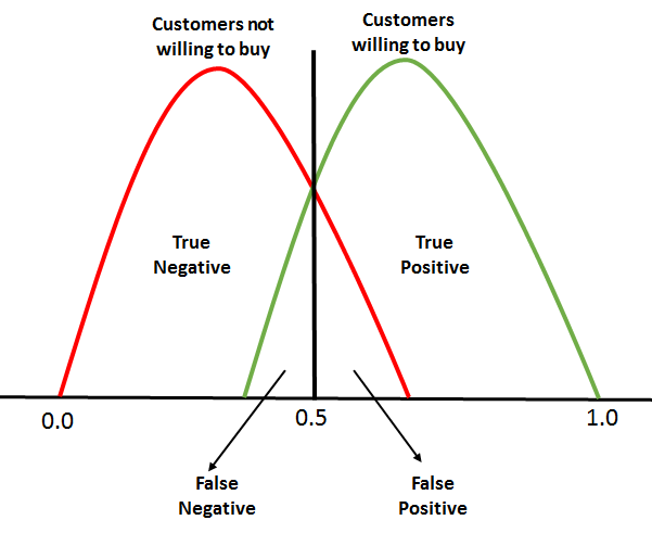
Most of the classifiers produce a score between 0 and 1. The next step occurs when we're setting up the threshold, and, based on this threshold, the classification is decided. Typically, 0.5 is the threshold—if it's more than 0.5, it creates a class, 1, and if the threshold is less than 0.5 it falls into another class, 2:

For ROC, every point between 0.0 and 1.0 is treated as a threshold, so the line of threshold keeps on moving from 0.0 to 1.0. The threshold will result in us having a TP, TN, FP, and FN. At every threshold, the following metrics are calculated:

  • True Positive Rate = TP/(TP+FN)

  • True Negative Rate = TN/(TN + FP)

  • False Positive Rate = 1- True Negative Rate

The calculation of (TPR and FPR) starts from 0. When the threshold line is at 0, we will be able to classify all of the customers who are willing to buy (positive cases), whereas those who are not willing to buy will be misclassified as there will be too many false positives. This means that the threshold line will start moving toward the right from zero. As this happens, the false positive starts to decline and the true positive will continue increasing.

Finally, we will need to plot a graph of the TPR versus FPR after calculating them at every point of the threshold:

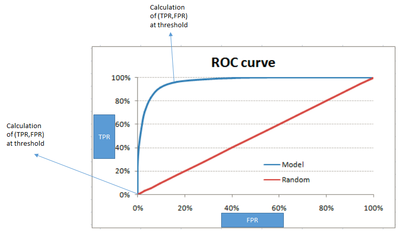
The red diagonal line represents the classification at random, that is, classification without the model. The perfect ROC curve will go along the y axis and will take the shape of an absolute triangle, which will pass through the top of the y axis. 

Area under ROC

To assess the model/classifier, we need to determine the area under ROC (AUROC). The whole area of this plot is 1 as the maximum value of FPR and TPR – both are 1 here. Hence, it takes the shape of a square. The random line is positioned perfectly at 45 degrees, which partitions the whole area into two symmetrical and equilateral triangles. This means that the areas under and above the red line are 0.5. The best and perfect classifier will be the one that tries to attain the AUROC as 1. The higher the AUROC, the better the model is.

In a situation where you have got multiple classifiers, you can use AUROC to determine which is the best one among the lot.

Visually different images
CONTINUE READING
83
Tech Concepts
36
Programming languages
73
Tech Tools
Icon Unlimited access to the largest independent learning library in tech of over 8,000 expert-authored tech books and videos.
Icon Innovative learning tools, including AI book assistants, code context explainers, and text-to-speech.
Icon 50+ new titles added per month and exclusive early access to books as they are being written.
Machine Learning Quick Reference
You have been reading a chapter from
Machine Learning Quick Reference
Published in: Jan 2019
Publisher: Packt
ISBN-13: 9781788830577
Register for a free Packt account to unlock a world of extra content!
A free Packt account unlocks extra newsletters, articles, discounted offers, and much more. Start advancing your knowledge today.
Unlock this book and the full library FREE for 7 days
Get unlimited access to 7000+ expert-authored eBooks and videos courses covering every tech area you can think of
Renews at $19.99/month. Cancel anytime
Modal Close icon
Modal Close icon