Curve fitting

So far, we have learned about the learning curve and its significance. However, it only comes into the picture once we tried fitting a curve on the available data and features. But what does curve fitting mean? Let's try to understand this.

Curve fitting is nothing but establishing a relationship between a number of features and a target. It helps in finding out what kind of association the features have with respect to the target. 

Establishing a relationship (curve fitting) is nothing but coming up with a mathematical function that should be able to explain the behavioral pattern in such a way that it comes across as a best fit for the dataset.

There are multiple reasons behind why we do curve fitting:

• To carry out system simulation and optimization
• To determine the values of intermediate points (interpolation)
• To do trend analysis (extrapolation)
• To carry out hypothesis testing

There are two types of curve fitting:

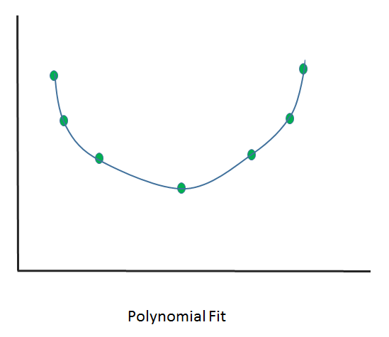
1. Exact fit: In this scenario, the curve would pass through all the points. There is no residual error (we'll discuss shortly what's classed as an error) in this case. For now, you can understand an error as the difference between the actual error and the predicted error. It can be used for interpolation and is majorly involved with a distribution fit. 

The following diagram shows the polynomial but exact fit:

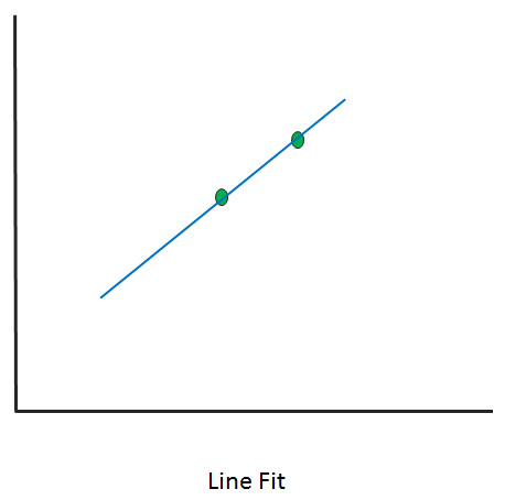
The following diagram shows the line but exact fit:

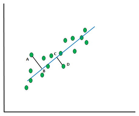
2. Best fit: The curve doesn't pass through all the points. There will be a residual associated with this.

Let's look at some different scenarios and study them to understand these differences.

Here, we will fit a curve for two numbers:

# importing libraries
 import numpy as np
 import matplotlib.pyplot as plt
 from scipy.optimize import curve_fit

# writing a function of Line
 def func(x, a, b):
 return a + b * x 
 x_d = np.linspace(0, 5, 2) # generating 2 numbers between 0 & 5
 y = func(x_d,1.5, 0.7) 
 y_noise = 0.3 * np.random.normal(size=x_d.size)
 y_d = y + y_noise
 plt.plot(x_d, y_d, 'b-', label='data')
 
 popt, pcov = curve_fit(func, x_d, y_d) # fitting the curve
 plt.plot(x_d, func(x_d, *popt), 'r-', label='fit')

From this, we will get the following output:

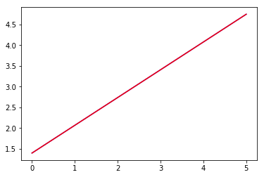
Here, we have used two points to fit the line and we can very well see that it becomes an exact fit. When introducing three points, we will get the following:

 x_d = np.linspace(0, 5, 3) # generating 3 numbers between 0 & 5

Run the entire code and focus on the output:

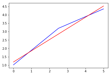
Now, you can see the drift and effect of noise. It has started to take the shape of a curve. A line might not be a good fit here (however, it's too early to say). It's no longer an exact fit.

What if we try to introduce 100 points and study the effect of that? By now, we know how to introduce the number of points.

By doing this, we get the following output:

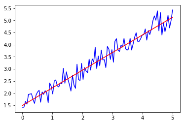
This is not an exact fit, but rather a best fit that tries to generalize the whole dataset.

Residual

Residuals are the difference between an observed or true value and a predicted (fitted) value. For example, in the following diagram, one of the residuals is (A-B), where A is the observed value and B is the fitted value:

The preceding scatter plot depicts that we are fitting a line that could represent the behavior of all the data points. However, one thing that's noticeable is that the line doesn't pass through all of the points. Most of the points are off the line.

The sum and mean of residuals will always be 0. ∑e =0 and mean of e =0.