Image I/O and display with Python

Images are stored as files on the disk, so reading and writing images from the files are disk I/O operations. These can be done using many ways using different libraries; some of them are shown in this section. Let us first start by importing all of the required packages:

# for inline image display inside notebook
# % matplotlib inline 
import numpy as np
from PIL import Image, ImageFont, ImageDraw
from PIL.ImageChops import add, subtract, multiply, difference, screen
import PIL.ImageStat as stat
from skimage.io import imread, imsave, imshow, show, imread_collection, imshow_collection
from skimage import color, viewer, exposure, img_as_float, data
from skimage.transform import SimilarityTransform, warp, swirl
from skimage.util import invert, random_noise, montage
import matplotlib.image as mpimg
import matplotlib.pylab as plt
from scipy.ndimage import affine_transform, zoom
from scipy import misc

 

 

 

 

Reading, saving, and displaying an image using PIL

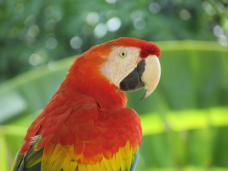
The PIL function, open(), reads an image from disk in an Image object, as shown in the following code. The image is loaded as an object of the PIL.PngImagePlugin.PngImageFileclass, and we can use properties such as the width, height, and mode to find the size (width x height in pixels or the resolution of the image) and mode of the image:

im = Image.open("../images/parrot.png") # read the image, provide the correct path
print(im.width, im.height, im.mode, im.format, type(im))
# 453 340 RGB PNG <class 'PIL.PngImagePlugin.PngImageFile'>
im.show() # display the image 

The following is the output of the previous code:

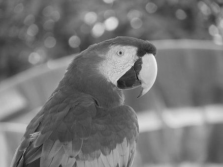
The following code block shows how to use the PIL function, convert(), to convert the colored RGB image into a grayscale image:

im_g = im.convert('L')                         # convert the RGB color image to a grayscale image
im_g.save('../images/parrot_gray.png')         # save the image to disk
Image.open("../images/parrot_gray.png").show() # read the grayscale image from disk and show

The following is the output grayscale image:

Providing the correct path to the images on the disk

We recommend creating a folder (sub-directory) to store images to be used for processing (for example, for the Python code samples, we have used the images stored inside a folder named images) and then provide the path to the folder to access the image to avoid the file not found exception.

Reading, saving, and displaying an image using Matplotlib

The next code block shows how to use the imread()function frommatplotlib.image to read an image in a floating-point numpy ndarray. The pixel values are represented as real values between 0 and 1:

im = mpimg.imread("../images/hill.png")  # read the image from disk as a numpy ndarray
print(im.shape, im.dtype, type(im))      # this image contains an α channel, hence num_channels= 4
# (960, 1280, 4) float32 <class 'numpy.ndarray'>
plt.figure(figsize=(10,10))
plt.imshow(im) # display the image
plt.axis('off')
plt.show()

The following figure shows the output of the previous code:

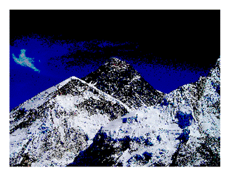
The next code snippet changes the image to a darker image by first setting all of the pixel values below 0.5 to 0 and then saving the numpy ndarray to disk. The saved image is again reloaded and displayed:

im1 = im 
im1[im1 < 0.5] = 0    # make the image look darker
plt.imshow(im1)
plt.axis('off')
plt.tight_layout()
plt.savefig("../images/hill_dark.png")       # save the dark image
im = mpimg.imread("../images/hill_dark.png") # read the dark image
plt.figure(figsize=(10,10))
plt.imshow(im)
plt.axis('off') # no axis ticks
plt.tight_layout()
plt.show()

The next figure shows the darker image saved with the preceding code: 

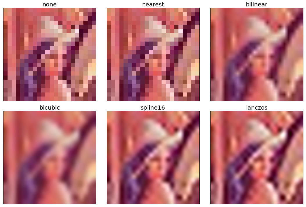
Interpolating while displaying with Matplotlib imshow()

The imshow() function from Matplotlib provides many different types of interpolation methods to plot an image. These functions can be particularly useful when the image to be plotted is small. Let us use the small 50 x 50 lena image shown in the next figure to see the effects of plotting with different interpolation methods:

 

The next code block demonstrates how to use different interpolation methods with imshow():

im = mpimg.imread("../images/lena_small.jpg") # read the image from disk as a numpy ndarray
methods = ['none', 'nearest', 'bilinear', 'bicubic', 'spline16', 'lanczos']
fig, axes = plt.subplots(nrows=2, ncols=3, figsize=(15, 30),
 subplot_kw={'xticks': [], 'yticks': []})
fig.subplots_adjust(hspace=0.05, wspace=0.05)
for ax, interp_method in zip(axes.flat, methods):
 ax.imshow(im, interpolation=interp_method)
 ax.set_title(str(interp_method), size=20)
plt.tight_layout()
plt.show()

The next figure shows the output of the preceding code:

Reading, saving, and displaying an image using scikit-image

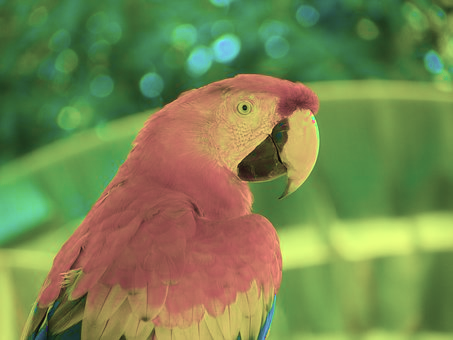
The next code block uses the imread()function fromscikit-image to read an image in a numpy ndarray of type uint8 (8-bit unsigned integer). Hence, the pixel values will be in between 0 and 255. Then it converts (changes the image type or mode, which will be discussed shortly) the colored RGB image into an HSV image using the hsv2rgb()function from the Image.color module. Next, it changes the saturation (colorfulness) to a constant value for all of the pixels by keeping the hue and value channels unchanged. The image is then converted back into RGB mode with the rgb2hsv() function to create a new image, which is then saved and displayed:

im = imread("../images/parrot.png")     # read image from disk, provide the correct path
print(im.shape, im.dtype, type(im)) 
# (362, 486, 3) uint8 <class 'numpy.ndarray'>
hsv = color.rgb2hsv(im) # from RGB to HSV color space
hsv[:, :, 1] = 0.5 # change the saturation
im1 = color.hsv2rgb(hsv) # from HSV back to RGB
imsave('../images/parrot_hsv.png', im1) # save image to disk
im = imread("../images/parrot_hsv.png")
plt.axis('off'), imshow(im), show()

The next figure shows the output of the previous code—a new image with changed saturation:

We can use the scikit-image viewer module also to display an image in a pop-up window, as shown in the following code:

viewer = viewer.ImageViewer(im)
viewer.show()

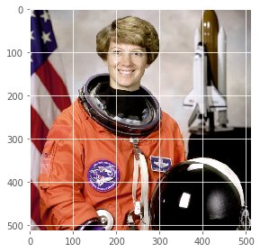
Using scikit-image's astronaut dataset

The following code block shows how we can load the astronaut image from the scikit-image library's image datasets with the data module. The module contains a few other popular datasets, such as cameraman, which can be loaded similarly:

im = data.astronaut() 
imshow(im), show()

 

 

 

 

 

 

The next figure shows the output of the preceding code:

Reading and displaying multiple images at once

We can use the imread_collection() function of the scikit-image io module to load in a folder all images that have a particular pattern in the filename and display them simultaneously with the imshow_collection() function. The code is left as an exercise for the reader.

Reading, saving, and displaying an image using scipy misc

The misc module of scipy can also be used for image I/O and display. The following sections demonstrate how to use the misc module functions.

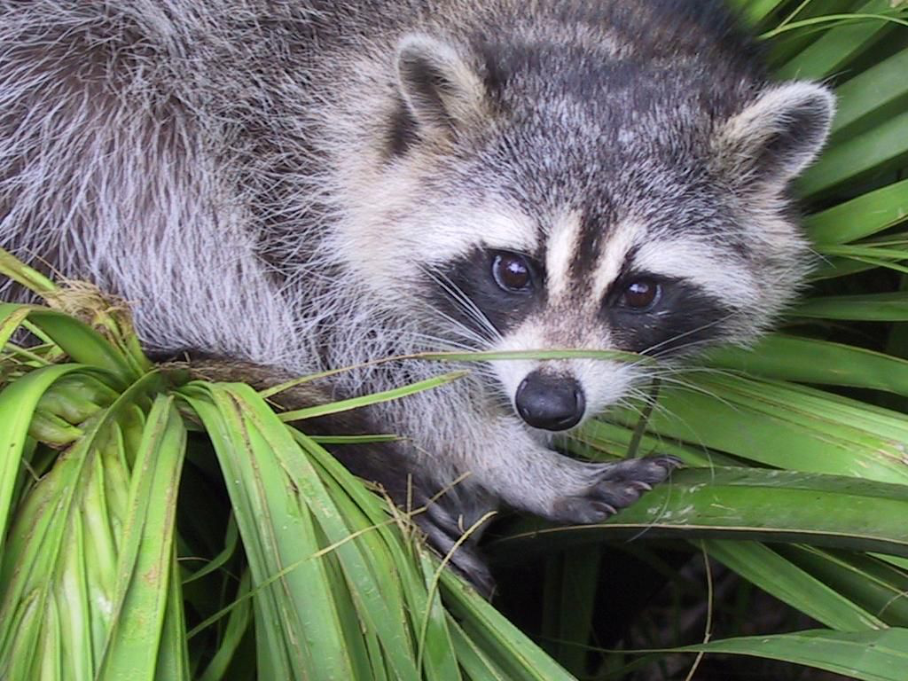
Using scipy.misc's face dataset

The next code block shows how to display the face dataset of the misc module:

im = misc.face() # load the raccoon's face image
misc.imsave('face.png', im) # uses the Image module (PIL)
plt.imshow(im), plt.axis('off'), plt.show()

 

 

The next figure shows the output of the previous code, which displays the misc module's face image:

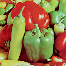
We can read an image from disk using misc.imread(). The next code block shows an example:

im = misc.imread('../images/pepper.jpg')
print(type(im), im.shape, im.dtype)
# <class 'numpy.ndarray'> (225, 225, 3) uint8

The I/O function's imread() is deprecated in SciPy 1.0.0, and will be removed in 1.2.0, so the documentation recommends we use the imageio library instead. The next code block shows how an image can be read with the imageio.imread() function and can be displayed with Matplotlib:

import imageio
im = imageio.imread('../images/pepper.jpg')
print(type(im), im.shape, im.dtype)
# <class 'imageio.core.util.Image'> (225, 225, 3) uint8
plt.imshow(im), plt.axis('off'), plt.show()

 

 

 

 

The next figure shows the output of the previous code block: