


 Download code from GitHub
In this chapter, you will learn basic data mining terms such as data definition, preprocessing, and so on.
The most important data mining algorithms will be illustrated with R to help you grasp the principles quickly, including but not limited to, classification, clustering, and outlier detection. Before diving right into data mining, let's have a look at the topics we'll cover:
- Data mining
- Social network mining
- Text mining
- Web data mining
- Why R
- Statistics
- Machine learning
- Data attributes and description
- Data measuring
- Data cleaning
- Data integration
- Data reduction
- Data transformation and discretization
- Visualization of results
In the history of humankind, the results of data from every aspect is extensive, for example websites, social networks by user's e-mail or name or account, search terms, locations on map, companies, IP addresses, books, films, music, and products.
Data mining techniques can be applied to any kind of old or emerging data; each data type can be best dealt with using certain, but not all, techniques. In other words, the data mining techniques are constrained by data type, size of the dataset, context of the tasks applied, and so on. Every dataset has its own appropriate data mining solutions.
New data mining techniques always need to be researched along with new data types once the old techniques cannot be applied to it or if the new data type cannot be transformed onto the traditional data types. The evolution of stream mining algorithms applied to Twitter's huge source set is one typical example. The graph mining algorithms developed for social networks is another example.
The most popular and basic forms of data are from databases, data warehouses, ordered/sequence data, graph data, text data, and so on. In other words, they are federated data, high dimensional data, longitudinal data, streaming data, web data, numeric, categorical, or text data.
Big data is large amount of data that does not fit in the memory of a single machine. In other words, the size of data itself becomes a part of the issue when studying it. Besides volume, two other major characteristics of big data are variety and velocity; these are the famous three Vs of big data. Velocity means data process rate or how fast the data is being processed. Variety denotes various data source types. Noises arise more frequently in big data source sets and affect the mining results, which require efficient data preprocessing algorithms.
As a result, distributed filesystems are used as tools for successful implementation of parallel algorithms on large amounts of data; it is a certainty that we will get even more data with each passing second. Data analytics and visualization techniques are the primary factors of the data mining tasks related to massive data. The characteristics of massive data appeal to many new data mining technique-related platforms, one of which is RHadoop. We'll be describing this in a later section.
Some data types that are important to big data are as follows:
- The data from the camera video, which includes more metadata for analysis to expedite crime investigations, enhanced retail analysis, military intelligence, and so on.
- The second data type is from embedded sensors, such as medical sensors, to monitor any potential outbreaks of virus.
- The third data type is from entertainment, information freely published through social media by anyone.
- The last data type is consumer images, aggregated from social medias, and tagging on these like images are important.
Here is a table illustrating the history of data size growth. It shows that information will be more than double every two years, changing the way researchers or companies manage and extract value through data mining techniques from data, revealing new data mining studies.
|
Year |
Data Sizes |
Comments |
|---|---|---|
|
N/A |
1 MB (Megabyte) = | |
|
N/A |
1 PB (Petabyte) = | |
|
1999 |
1 EB |
1 EB (Exabyte) = |
|
2007 |
281 EB |
The world produced about 281 Exabyte of unique information. |
|
2011 |
1.8 ZB |
1 ZB (Zetabyte)= |
|
Very soon |
1 YB(Yottabytes)= |


Efficiency, scalability, performance, optimization, and the ability to perform in real time are important issues for almost any algorithms, and it is the same for data mining. There are always necessary metrics or benchmark factors of data mining algorithms.
As the amount of data continues to grow, keeping data mining algorithms effective and scalable is necessary to effectively extract information from massive datasets in many data repositories or data streams.
The storage of data from a single machine to wide distribution, the huge size of many datasets, and the computational complexity of the data mining methods are all factors that drive the development of parallel and distributed data-intensive mining algorithms.
Data serves as the input for the data mining system and data repositories are important. In an enterprise environment, database and logfiles are common sources. In web data mining, web pages are the source of data. The data that continuously fetched various sensors are also a typical data source.
Note
Here are some free online data sources particularly helpful to learn about data mining:
- Frequent Itemset Mining Dataset Repository: A repository with datasets for methods to find frequent itemsets (http://fimi.ua.ac.be/data/).
- UCI Machine Learning Repository: This is a collection of dataset, suitable for classification tasks (http://archive.ics.uci.edu/ml/).
- The Data and Story Library at statlib: DASL (pronounced "dazzle") is an online library of data files and stories that illustrate the use of basic statistics methods. We hope to provide data from a wide variety of topics so that statistics teachers can find real-world examples that will be interesting to their students. Use DASL's powerful search engine to locate the story or data file of interest. (http://lib.stat.cmu.edu/DASL/)
- WordNet: This is a lexical database for English (http://wordnet.princeton.edu)
Data mining is the discovery of a model in data; it's also called exploratory data analysis, and discovers useful, valid, unexpected, and understandable knowledge from the data. Some goals are shared with other sciences, such as statistics, artificial intelligence, machine learning, and pattern recognition. Data mining has been frequently treated as an algorithmic problem in most cases. Clustering, classification, association rule learning, anomaly detection, regression, and summarization are all part of the tasks belonging to data mining.
The data mining methods can be summarized into two main categories of data mining problems: feature extraction and summarization.
This is to extract the most prominent features of the data and ignore the rest. Here are some examples:
- Frequent itemsets: This model makes sense for data that consists of baskets of small sets of items.
- Similar items: Sometimes your data looks like a collection of sets and the objective is to find pairs of sets that have a relatively large fraction of their elements in common. It's a fundamental problem of data mining.
The target is to summarize the dataset succinctly and approximately, such as clustering, which is the process of examining a collection of points (data) and grouping the points into clusters according to some measure. The goal is that points in the same cluster have a small distance from one another, while points in different clusters are at a large distance from one another.
There are two popular processes to define the data mining process in different perspectives, and the more widely adopted one is CRISP-DM:
There are six phases in this process that are shown in the following figure; it is not rigid, but often has a great deal of backtracking:

Let's look at the phases in detail:
- Business understanding: This task includes determining business objectives, assessing the current situation, establishing data mining goals, and developing a plan.
- Data understanding: This task evaluates data requirements and includes initial data collection, data description, data exploration, and the verification of data quality.
- Data preparation: Once available, data resources are identified in the last step. Then, the data needs to be selected, cleaned, and then built into the desired form and format.
- Modeling: Visualization and cluster analysis are useful for initial analysis. The initial association rules can be developed by applying tools such as generalized rule induction. This is a data mining technique to discover knowledge represented as rules to illustrate the data in the view of causal relationship between conditional factors and a given decision/outcome. The models appropriate to the data type can also be applied.
- Evaluation :The results should be evaluated in the context specified by the business objectives in the first step. This leads to the identification of new needs and in turn reverts to the prior phases in most cases.
- Deployment: Data mining can be used to both verify previously held hypotheses or for knowledge.
Here is an overview of the process for SEMMA:

Let's look at these processes in detail:
- Sample: In this step, a portion of a large dataset is extracted
- Explore: To gain a better understanding of the dataset, unanticipated trends and anomalies are searched in this step
- Modify: The variables are created, selected, and transformed to focus on the model construction process
- Model: A variable combination of models is searched to predict a desired outcome
- Assess: The findings from the data mining process are evaluated by its usefulness and reliability
Feature extraction
This is to extract the most prominent features of the data and ignore the rest. Here are some examples:
- Frequent itemsets: This model makes sense for data that consists of baskets of small sets of items.
- Similar items: Sometimes your data looks like a collection of sets and the objective is to find pairs of sets that have a relatively large fraction of their elements in common. It's a fundamental problem of data mining.
The target is to summarize the dataset succinctly and approximately, such as clustering, which is the process of examining a collection of points (data) and grouping the points into clusters according to some measure. The goal is that points in the same cluster have a small distance from one another, while points in different clusters are at a large distance from one another.
There are two popular processes to define the data mining process in different perspectives, and the more widely adopted one is CRISP-DM:
There are six phases in this process that are shown in the following figure; it is not rigid, but often has a great deal of backtracking:
Let's look at the phases in detail:
- Business understanding: This task includes determining business objectives, assessing the current situation, establishing data mining goals, and developing a plan.
- Data understanding: This task evaluates data requirements and includes initial data collection, data description, data exploration, and the verification of data quality.
- Data preparation: Once available, data resources are identified in the last step. Then, the data needs to be selected, cleaned, and then built into the desired form and format.
- Modeling: Visualization and cluster analysis are useful for initial analysis. The initial association rules can be developed by applying tools such as generalized rule induction. This is a data mining technique to discover knowledge represented as rules to illustrate the data in the view of causal relationship between conditional factors and a given decision/outcome. The models appropriate to the data type can also be applied.
- Evaluation :The results should be evaluated in the context specified by the business objectives in the first step. This leads to the identification of new needs and in turn reverts to the prior phases in most cases.
- Deployment: Data mining can be used to both verify previously held hypotheses or for knowledge.
Here is an overview of the process for SEMMA:
Let's look at these processes in detail:
- Sample: In this step, a portion of a large dataset is extracted
- Explore: To gain a better understanding of the dataset, unanticipated trends and anomalies are searched in this step
- Modify: The variables are created, selected, and transformed to focus on the model construction process
- Model: A variable combination of models is searched to predict a desired outcome
- Assess: The findings from the data mining process are evaluated by its usefulness and reliability
Summarization
The target is to summarize the dataset succinctly and approximately, such as clustering, which is the process of examining a collection of points (data) and grouping the points into clusters according to some measure. The goal is that points in the same cluster have a small distance from one another, while points in different clusters are at a large distance from one another.
There are two popular processes to define the data mining process in different perspectives, and the more widely adopted one is CRISP-DM:
There are six phases in this process that are shown in the following figure; it is not rigid, but often has a great deal of backtracking:
Let's look at the phases in detail:
- Business understanding: This task includes determining business objectives, assessing the current situation, establishing data mining goals, and developing a plan.
- Data understanding: This task evaluates data requirements and includes initial data collection, data description, data exploration, and the verification of data quality.
- Data preparation: Once available, data resources are identified in the last step. Then, the data needs to be selected, cleaned, and then built into the desired form and format.
- Modeling: Visualization and cluster analysis are useful for initial analysis. The initial association rules can be developed by applying tools such as generalized rule induction. This is a data mining technique to discover knowledge represented as rules to illustrate the data in the view of causal relationship between conditional factors and a given decision/outcome. The models appropriate to the data type can also be applied.
- Evaluation :The results should be evaluated in the context specified by the business objectives in the first step. This leads to the identification of new needs and in turn reverts to the prior phases in most cases.
- Deployment: Data mining can be used to both verify previously held hypotheses or for knowledge.
Here is an overview of the process for SEMMA:
Let's look at these processes in detail:
- Sample: In this step, a portion of a large dataset is extracted
- Explore: To gain a better understanding of the dataset, unanticipated trends and anomalies are searched in this step
- Modify: The variables are created, selected, and transformed to focus on the model construction process
- Model: A variable combination of models is searched to predict a desired outcome
- Assess: The findings from the data mining process are evaluated by its usefulness and reliability
The data mining process
There are two popular processes to define the data mining process in different perspectives, and the more widely adopted one is CRISP-DM:
There are six phases in this process that are shown in the following figure; it is not rigid, but often has a great deal of backtracking:
Let's look at the phases in detail:
- Business understanding: This task includes determining business objectives, assessing the current situation, establishing data mining goals, and developing a plan.
- Data understanding: This task evaluates data requirements and includes initial data collection, data description, data exploration, and the verification of data quality.
- Data preparation: Once available, data resources are identified in the last step. Then, the data needs to be selected, cleaned, and then built into the desired form and format.
- Modeling: Visualization and cluster analysis are useful for initial analysis. The initial association rules can be developed by applying tools such as generalized rule induction. This is a data mining technique to discover knowledge represented as rules to illustrate the data in the view of causal relationship between conditional factors and a given decision/outcome. The models appropriate to the data type can also be applied.
- Evaluation :The results should be evaluated in the context specified by the business objectives in the first step. This leads to the identification of new needs and in turn reverts to the prior phases in most cases.
- Deployment: Data mining can be used to both verify previously held hypotheses or for knowledge.
Here is an overview of the process for SEMMA:
Let's look at these processes in detail:
- Sample: In this step, a portion of a large dataset is extracted
- Explore: To gain a better understanding of the dataset, unanticipated trends and anomalies are searched in this step
- Modify: The variables are created, selected, and transformed to focus on the model construction process
- Model: A variable combination of models is searched to predict a desired outcome
- Assess: The findings from the data mining process are evaluated by its usefulness and reliability
CRISP-DM
There are six phases in this process that are shown in the following figure; it is not rigid, but often has a great deal of backtracking:
Let's look at the phases in detail:
- Business understanding: This task includes determining business objectives, assessing the current situation, establishing data mining goals, and developing a plan.
- Data understanding: This task evaluates data requirements and includes initial data collection, data description, data exploration, and the verification of data quality.
- Data preparation: Once available, data resources are identified in the last step. Then, the data needs to be selected, cleaned, and then built into the desired form and format.
- Modeling: Visualization and cluster analysis are useful for initial analysis. The initial association rules can be developed by applying tools such as generalized rule induction. This is a data mining technique to discover knowledge represented as rules to illustrate the data in the view of causal relationship between conditional factors and a given decision/outcome. The models appropriate to the data type can also be applied.
- Evaluation :The results should be evaluated in the context specified by the business objectives in the first step. This leads to the identification of new needs and in turn reverts to the prior phases in most cases.
- Deployment: Data mining can be used to both verify previously held hypotheses or for knowledge.
Here is an overview of the process for SEMMA:
Let's look at these processes in detail:
- Sample: In this step, a portion of a large dataset is extracted
- Explore: To gain a better understanding of the dataset, unanticipated trends and anomalies are searched in this step
- Modify: The variables are created, selected, and transformed to focus on the model construction process
- Model: A variable combination of models is searched to predict a desired outcome
- Assess: The findings from the data mining process are evaluated by its usefulness and reliability
SEMMA
Here is an overview of the process for SEMMA:
Let's look at these processes in detail:
- Sample: In this step, a portion of a large dataset is extracted
- Explore: To gain a better understanding of the dataset, unanticipated trends and anomalies are searched in this step
- Modify: The variables are created, selected, and transformed to focus on the model construction process
- Model: A variable combination of models is searched to predict a desired outcome
- Assess: The findings from the data mining process are evaluated by its usefulness and reliability
As we mentioned before, data mining finds a model on data and the mining of social network finds the model on graph data in which the social network is represented.
Social network mining is one application of web data mining; the popular applications are social sciences and bibliometry, PageRank and HITS, shortcomings of the coarse-grained graph model, enhanced models and techniques, evaluation of topic distillation, and measuring and modeling the Web.
When it comes to the discussion of social networks, you will think of Facebook, Google+, LinkedIn, and so on. The essential characteristics of a social network are as follows:
- There is a collection of entities that participate in the network. Typically, these entities are people, but they could be something else entirely.
- There is at least one relationship between the entities of the network. On Facebook, this relationship is called friends. Sometimes, the relationship is all-or-nothing; two people are either friends or they are not. However, in other examples of social networks, the relationship has a degree. This degree could be discrete, for example, friends, family, acquaintances, or none as in Google+. It could be a real number; an example would be the fraction of the average day that two people spend talking to each other.
- There is an assumption of nonrandomness or locality. This condition is the hardest to formalize, but the intuition is that relationships tend to cluster. That is, if entity A is related to both B and C, then there is a higher probability than average that B and C are related.
Here are some varieties of social networks:
- Telephone networks: The nodes in this network are phone numbers and represent individuals
- E-mail networks: The nodes represent e-mail addresses, which represent individuals
- Collaboration networks: The nodes here represent individuals who published research papers; the edge connecting two nodes represent two individuals who published one or more papers jointly
Social networks are modeled as undirected graphs. The entities are the nodes, and an edge connects two nodes if the nodes are related by the relationship that characterizes the network. If there is a degree associated with the relationship, this degree is represented by labeling the edges.

Here is an example in which Coleman's High School Friendship Data from the sna R package is used for analysis. The data is from a research on friendship ties between 73 boys in a high school in one chosen academic year; reported ties for all informants are provided for two time points (fall and spring). The dataset's name is coleman, which is an array type in R language. The node denotes a specific student and the line represents the tie between two students.

Social network
When it comes to the discussion of social networks, you will think of Facebook, Google+, LinkedIn, and so on. The essential characteristics of a social network are as follows:
- There is a collection of entities that participate in the network. Typically, these entities are people, but they could be something else entirely.
- There is at least one relationship between the entities of the network. On Facebook, this relationship is called friends. Sometimes, the relationship is all-or-nothing; two people are either friends or they are not. However, in other examples of social networks, the relationship has a degree. This degree could be discrete, for example, friends, family, acquaintances, or none as in Google+. It could be a real number; an example would be the fraction of the average day that two people spend talking to each other.
- There is an assumption of nonrandomness or locality. This condition is the hardest to formalize, but the intuition is that relationships tend to cluster. That is, if entity A is related to both B and C, then there is a higher probability than average that B and C are related.
Here are some varieties of social networks:
- Telephone networks: The nodes in this network are phone numbers and represent individuals
- E-mail networks: The nodes represent e-mail addresses, which represent individuals
- Collaboration networks: The nodes here represent individuals who published research papers; the edge connecting two nodes represent two individuals who published one or more papers jointly
Social networks are modeled as undirected graphs. The entities are the nodes, and an edge connects two nodes if the nodes are related by the relationship that characterizes the network. If there is a degree associated with the relationship, this degree is represented by labeling the edges.
Here is an example in which Coleman's High School Friendship Data from the sna R package is used for analysis. The data is from a research on friendship ties between 73 boys in a high school in one chosen academic year; reported ties for all informants are provided for two time points (fall and spring). The dataset's name is coleman, which is an array type in R language. The node denotes a specific student and the line represents the tie between two students.
Text mining is based on the data of text, concerned with exacting relevant information from large natural language text, and searching for interesting relationships, syntactical correlation, or semantic association between the extracted entities or terms. It is also defined as automatic or semiautomatic processing of text. The related algorithms include text clustering, text classification, natural language processing, and web mining.
One of the characteristics of text mining is text mixed with numbers, or in other point of view, the hybrid data type contained in the source dataset. The text is usually a collection of unstructured documents, which will be preprocessed and transformed into a numerical and structured representation. After the transformation, most of the data mining algorithms can be applied with good effects.
The process of text mining is described as follows:
- Text mining starts from preparing the text corpus, which are reports, letters and so forth
- The second step is to build a semistructured text database that is based on the text corpus
- The third step is to build a term-document matrix in which the term frequency is included
- The final result is further analysis, such as text analysis, semantic analysis, information retrieval, and information summarization
Information retrieval is to help users find information, most commonly associated with online documents. It focuses on the acquisition, organization, storage, retrieval, and distribution for information. The task of Information Retrieval (IR) is to retrieve relevant documents in response to a query. The fundamental technique of IR is measuring similarity. Key steps in IR are as follows:
- Specify a query. The following are some of the types of queries:
- Keyword query: This is expressed by a list of keywords to find documents that contain at least one keyword
- Boolean query: This is constructed with Boolean operators and keywords
- Phrase query: This is a query that consists of a sequence of words that makes up a phrase
- Proximity query: This is a downgrade version of the phrase queries and can be a combination of keywords and phrases
- Full document query: This query is a full document to find other documents similar to the query document
- Natural language questions: This query helps to express users' requirements as a natural language question
- Search the document collection.
- Return the subset of relevant documents.
Prediction of results from text is just as ambitious as predicting numerical data mining and has similar problems associated with numerical classification. It is generally a classification issue.
Prediction from text needs prior experience, from the sample, to learn how to draw a prediction on new documents. Once text is transformed into numeric data, prediction methods can be applied.
Information retrieval and text mining
Information retrieval is to help users find information, most commonly associated with online documents. It focuses on the acquisition, organization, storage, retrieval, and distribution for information. The task of Information Retrieval (IR) is to retrieve relevant documents in response to a query. The fundamental technique of IR is measuring similarity. Key steps in IR are as follows:
- Specify a query. The following are some of the types of queries:
- Keyword query: This is expressed by a list of keywords to find documents that contain at least one keyword
- Boolean query: This is constructed with Boolean operators and keywords
- Phrase query: This is a query that consists of a sequence of words that makes up a phrase
- Proximity query: This is a downgrade version of the phrase queries and can be a combination of keywords and phrases
- Full document query: This query is a full document to find other documents similar to the query document
- Natural language questions: This query helps to express users' requirements as a natural language question
- Search the document collection.
- Return the subset of relevant documents.
Prediction of results from text is just as ambitious as predicting numerical data mining and has similar problems associated with numerical classification. It is generally a classification issue.
Prediction from text needs prior experience, from the sample, to learn how to draw a prediction on new documents. Once text is transformed into numeric data, prediction methods can be applied.
Mining text for prediction
Prediction of results from text is just as ambitious as predicting numerical data mining and has similar problems associated with numerical classification. It is generally a classification issue.
Prediction from text needs prior experience, from the sample, to learn how to draw a prediction on new documents. Once text is transformed into numeric data, prediction methods can be applied.
Web mining aims to discover useful information or knowledge from the web hyperlink structure, page, and usage data. The Web is one of the biggest data sources to serve as the input for data mining applications.
Web data mining is based on IR, machine learning (ML), statistics, pattern recognition, and data mining. Web mining is not purely a data mining problem because of the heterogeneous and semistructured or unstructured web data, although many data mining approaches can be applied to it.
Web mining tasks can be defined into at least three types:
- Web structure mining: This helps to find useful information or valuable structural summary about sites and pages from hyperlinks
- Web content mining: This helps to mine useful information from web page contents
- Web usage mining: This helps to discover user access patterns from web logs to detect intrusion, fraud, and attempted break-in
The algorithms applied to web data mining are originated from classical data mining algorithms. They share many similarities, such as the mining process; however, differences exist too. The characteristics of web data mining makes it different from data mining for the following reasons:
- The data is unstructured
- The information of the Web keeps changing and the amount of data keeps growing
- Any data type is available on the Web, such as structured and unstructured data
- Heterogeneous information is on the web; redundant pages are present too
- Vast amounts of information on the web is linked
- The data is noisy
Web data mining differentiates from data mining by the huge dynamic volume of source dataset, a big variety of data format, and so on. The most popular data mining tasks related to the Web are as follows:
- Information extraction (IE): The task of IE consists of a couple of steps, tokenization, sentence segmentation, part-of-speech assignment, named entity identification, phrasal parsing, sentential parsing, semantic interpretation, discourse interpretation, template filling, and merging.
- Natural language processing (NLP): This researches the linguistic characteristics of human-human and human-machine interactive, models of linguistic competence and performance, frameworks to implement process with such models, processes'/models' iterative refinement, and evaluation techniques for the result systems. Classical NLP tasks related to web data mining are tagging, knowledge representation, ontologies, and so on.
- Question answering: The goal is to find the answer from a collection of text to questions in natural language format. It can be categorized into slot filling, limited domain, and open domain with bigger difficulties for the latter. One simple example is based on a predefined FAQ to answer queries from customers.
- Resource discovery: The popular applications are collecting important pages preferentially; similarity search using link topology, topical locality and focused crawling; and discovering communities.
R is a high-quality, cross-platform, flexible, widely used open source, free language for statistics, graphics, mathematics, and data science—created by statisticians for statisticians.
R contains more than 5,000 algorithms and millions of users with domain knowledge worldwide, and it is supported by a vibrant and talented community of contributors. It allows access to both well-established and experimental statistical techniques.
R is a free, open source software environment maintained by R-projects for statistical computing and graphics, and the R source code is available under the terms of the Free Software Foundation's GNU General Public License. R compiles and runs on a wide variety for a variety of platforms, such as UNIX, LINUX, Windows, and Mac OS.
There are three shortages of R:
- One is that it is memory bound, so it requires the entire dataset store in memory (RAM) to achieve high performance, which is also called in-memory analytics.
- Similar to other open source systems, anyone can create and contribute package with strict or less testing. In other words, packages contributing to R communities are bug-prone and need more testing to ensure the quality of codes.
- R seems slow than some other commercial languages.
Fortunately, there are packages available to overcome these problems. There are some solutions that can be categorized as parallelism solutions; the essence here is to spread work across multiple CPUs that overcome the R shortages that were just listed. Good examples include, but are not limited to, RHadoop. You will read more on this topic soon in the following sections. You can download the SNOW add-on package and the Parallel add-on package from Comprehensive R Archive Network (CRAN).
What are the disadvantages of R?
There are three shortages of R:
- One is that it is memory bound, so it requires the entire dataset store in memory (RAM) to achieve high performance, which is also called in-memory analytics.
- Similar to other open source systems, anyone can create and contribute package with strict or less testing. In other words, packages contributing to R communities are bug-prone and need more testing to ensure the quality of codes.
- R seems slow than some other commercial languages.
Fortunately, there are packages available to overcome these problems. There are some solutions that can be categorized as parallelism solutions; the essence here is to spread work across multiple CPUs that overcome the R shortages that were just listed. Good examples include, but are not limited to, RHadoop. You will read more on this topic soon in the following sections. You can download the SNOW add-on package and the Parallel add-on package from Comprehensive R Archive Network (CRAN).
Statistics studies the collection, analysis, interpretation or explanation, and presentation of data. It serves as the foundation of data mining and the relations will be illustrated in the following sections.
Statisticians were the first to use the term data mining. Originally, data mining was a derogatory term referring to attempts to extract information that was not supported by the data. To some extent, data mining constructs statistical models, which is an underlying distribution, used to visualize data.
Data mining has an inherent relationship with statistics; one of the mathematical foundations of data mining is statistics, and many statistics models are used in data mining.
Statistical methods can be used to summarize a collection of data and can also be used to verify data mining results.
Along with the development of statistics and machine learning, there is a continuum between these two subjects. Statistical tests are used to validate the machine learning models and to evaluate machine learning algorithms. Machine learning techniques are incorporated with standard statistical techniques.
R is a statistical programming language. It provides a huge amount of statistical functions, which are based on the knowledge of statistics. Many R add-on package contributors come from the field of statistics and use R in their research.
During the evolution of data mining technologies, due to statistical limits on data mining, one can make errors by trying to extract what really isn't in the data.
Bonferroni's Principle is a statistical theorem otherwise known as Bonferroni correction. You can assume that big portions of the items you find are bogus, that is, the items returned by the algorithms dramatically exceed what is assumed.
Statistics and data mining
Statisticians were the first to use the term data mining. Originally, data mining was a derogatory term referring to attempts to extract information that was not supported by the data. To some extent, data mining constructs statistical models, which is an underlying distribution, used to visualize data.
Data mining has an inherent relationship with statistics; one of the mathematical foundations of data mining is statistics, and many statistics models are used in data mining.
Statistical methods can be used to summarize a collection of data and can also be used to verify data mining results.
Along with the development of statistics and machine learning, there is a continuum between these two subjects. Statistical tests are used to validate the machine learning models and to evaluate machine learning algorithms. Machine learning techniques are incorporated with standard statistical techniques.
R is a statistical programming language. It provides a huge amount of statistical functions, which are based on the knowledge of statistics. Many R add-on package contributors come from the field of statistics and use R in their research.
During the evolution of data mining technologies, due to statistical limits on data mining, one can make errors by trying to extract what really isn't in the data.
Bonferroni's Principle is a statistical theorem otherwise known as Bonferroni correction. You can assume that big portions of the items you find are bogus, that is, the items returned by the algorithms dramatically exceed what is assumed.
Statistics and machine learning
Along with the development of statistics and machine learning, there is a continuum between these two subjects. Statistical tests are used to validate the machine learning models and to evaluate machine learning algorithms. Machine learning techniques are incorporated with standard statistical techniques.
R is a statistical programming language. It provides a huge amount of statistical functions, which are based on the knowledge of statistics. Many R add-on package contributors come from the field of statistics and use R in their research.
During the evolution of data mining technologies, due to statistical limits on data mining, one can make errors by trying to extract what really isn't in the data.
Bonferroni's Principle is a statistical theorem otherwise known as Bonferroni correction. You can assume that big portions of the items you find are bogus, that is, the items returned by the algorithms dramatically exceed what is assumed.
Statistics and R
R is a statistical programming language. It provides a huge amount of statistical functions, which are based on the knowledge of statistics. Many R add-on package contributors come from the field of statistics and use R in their research.
During the evolution of data mining technologies, due to statistical limits on data mining, one can make errors by trying to extract what really isn't in the data.
Bonferroni's Principle is a statistical theorem otherwise known as Bonferroni correction. You can assume that big portions of the items you find are bogus, that is, the items returned by the algorithms dramatically exceed what is assumed.
The limitations of statistics on data mining
During the evolution of data mining technologies, due to statistical limits on data mining, one can make errors by trying to extract what really isn't in the data.
Bonferroni's Principle is a statistical theorem otherwise known as Bonferroni correction. You can assume that big portions of the items you find are bogus, that is, the items returned by the algorithms dramatically exceed what is assumed.
The data to which a ML algorithm is applied is called a training set, which consists of a set of pairs (x, y), called training examples. The pairs are explained as follows:
x: This is a vector of values, often called the feature vector. Each value, or feature, can be categorical (values are taken from a set of discrete values, such as{S, M, L}) or numerical.y: This is the label, the classification or regression values forx.
The objective of the ML process is to discover a function  that best predicts the value of
 y associated with each value of x. The type of y is in principle arbitrary, but there are several common and important cases.
y: This is a real number. The ML problem is called regression.y: This is a Boolean value true or false, more commonly written as +1 and -1, respectively. In this class, the problem is binary classification.y: Here this is a member of some finite set. The member of this set can be thought of as classes, and each member represents one class. The problem is multiclass classification.y: This is a member of some potentially infinite set, for example, a parse tree forx, which is interpreted as a sentence.
Until now, machine learning has not proved successful in situations where we can describe the goals of the mining more directly. Machine learning and data mining are two different topics, although some algorithms are shared between them—algorithms are shared especially when the goal is to extract information. There are situations where machine learning makes sense. The typical one is when we have idea of what we looking for in the dataset.
The major classes of algorithms are listed here. Each is distinguished by the function  .
.
- Decision tree: This form of is a tree and each node of the tree has a function of
xthat determines which child or children the search must proceed for. - Perceptron: These are threshold functions applied to the components of the vector
 . A weight
  is associated with the ith components, for each i = 1, 2, … n, and there is a threshold
  . The output is +1 if and the output is -1 otherwise.
- Neural nets: These are acyclic networks of perceptions, with the outputs of some perceptions used as inputs to others.
- Instance-based learning: This uses the entire training set to represent the function .
- Support-vector machines: The result of this class is a classifier that tends to be more accurate on unseen data. The target for class separation denotes as looking for the optimal hyper-plane separating two classes by maximizing the margin between the classes' closest points.
The data aspects of machine learning here means the way data is handled and the way it is used to build the model.
- Training and testing: Assuming all the data is suitable for training, separate out a small fraction of the available data as the test set; use the remaining data to build a suitable model or classifier.
- Batch versus online learning: The entire training set is available at the beginning of the process for batch mode; the other one is online learning, where the training set arrives in a stream and cannot be revisited after it is processed.
- Feature selection: This helps to figure out what features to use as input to the learning algorithm.
- Creating a training set: This helps to create the label information that turns data into a training set by hand.
Approaches to machine learning
The major classes of algorithms are listed here. Each is distinguished by the function .
- Decision tree: This form of is a tree and each node of the tree has a function of
xthat determines which child or children the search must proceed for. - Perceptron: These are threshold functions applied to the components of the vector . A weight is associated with the ith components, for each i = 1, 2, … n, and there is a threshold . The output is +1 if and the output is -1 otherwise.
- Neural nets: These are acyclic networks of perceptions, with the outputs of some perceptions used as inputs to others.
- Instance-based learning: This uses the entire training set to represent the function .
- Support-vector machines: The result of this class is a classifier that tends to be more accurate on unseen data. The target for class separation denotes as looking for the optimal hyper-plane separating two classes by maximizing the margin between the classes' closest points.
The data aspects of machine learning here means the way data is handled and the way it is used to build the model.
- Training and testing: Assuming all the data is suitable for training, separate out a small fraction of the available data as the test set; use the remaining data to build a suitable model or classifier.
- Batch versus online learning: The entire training set is available at the beginning of the process for batch mode; the other one is online learning, where the training set arrives in a stream and cannot be revisited after it is processed.
- Feature selection: This helps to figure out what features to use as input to the learning algorithm.
- Creating a training set: This helps to create the label information that turns data into a training set by hand.
Machine learning architecture
The data aspects of machine learning here means the way data is handled and the way it is used to build the model.
- Training and testing: Assuming all the data is suitable for training, separate out a small fraction of the available data as the test set; use the remaining data to build a suitable model or classifier.
- Batch versus online learning: The entire training set is available at the beginning of the process for batch mode; the other one is online learning, where the training set arrives in a stream and cannot be revisited after it is processed.
- Feature selection: This helps to figure out what features to use as input to the learning algorithm.
- Creating a training set: This helps to create the label information that turns data into a training set by hand.
An attribute is a field representing a certain feature, characteristic, or dimensions of a data object.
In most situations, data can be modeled or represented with a matrix, columns for data attributes, and rows for certain data records in the dataset. For other cases, that data cannot be represented with matrices, such as text, time series, images, audio, video, and so forth. The data can be transformed into a matrix by appropriate methods, such as feature extraction.
The type of data attributes arises from its contexts or domains or semantics, and there are numerical, non-numerical, categorical data types or text data. Two views applied to data attributes and descriptions are widely used in data mining and R. They are as follows:
- Data in algebraic or geometric view: The entire dataset can be modeled into a matrix; linear algebraic and abstract algebra plays an important role here.
- Data in probability view: The observed data is treated as multidimensional random variables; each numeric attribute is a random variable. The dimension is the data dimension. Irrespective of whether the value is discrete or continuous, the probability theory can be applied here.
To help you learn R more naturally, we shall adopt a geometric, algebraic, and probabilistic view of the data.
Here is a matrix example. The number of columns is determined by m, which is the dimensionality of data. The number of rows is determined by n, which is the size of dataset.

Where  denotes the i row, which is an m-tuple as follows:

And  denotes the j column, which is an n-tuple as follows:

Numerical data is convenient to deal with because it is quantitative and allows arbitrary calculations. The properties of numerical data are the same as integer or float data.
Numeric attributes taken from a finite or countable infinite set of values are called discrete, for example a human being's age, which is the integer value starting from 1,150. Other attributes taken from any real values are called continuous. There are two main kinds of numeric types:
- Interval-scaled: This is the quantitative value, measured on a scale of equal unit, such as the weight of some certain fish in the scale of international metric, such as gram or kilogram.
- Ratio-scaled: This value can be computed by ratios between values in addition to differences between values. It is a numeric attribute with an inherent zero-point; hence, we can say a value is a multiple of another value.
The values of categorical attributes come from a set-valued domain composed of a set of symbols, such as the size of human costumes that are categorized as {S, M, L}. The categorical attributes can be divided into two groups or types:
The basic description can be used to identify features of data, distinguish noise, or outliers. A couple of basic statistical descriptions are as follows:
Data measuring is used in clustering, outlier detection, and classification. It refers to measures of proximity, similarity, and dissimilarity. The similarity value, a real value, between two tuples or data records ranges from 0 to 1, the higher the value the greater the similarity between tuples. Dissimilarity works in the opposite way; the higher the dissimilarity value, the more dissimilar are the two tuples.
For a dataset, data matrix stores the n data tuples in n x m matrix (n tuples and m attributes):

The dissimilarity matrix stores a collection of proximities available for all n tuples in the dataset, often in a n x n matrix. In the following matrix,  means the dissimilarity between two tuples; value 0 for highly similar or near between each other, 1 for completely same, the higher the value, the more dissimilar it is.

Most of the time, the dissimilarity and similarity are related concepts. The similarity measure can often be defined using a function; the expression constructed with measures of dissimilarity, and vice versa.
Here is a table with a list of some of the most used measures for different attribute value types:
Numeric attributes
Numerical data is convenient to deal with because it is quantitative and allows arbitrary calculations. The properties of numerical data are the same as integer or float data.
Numeric attributes taken from a finite or countable infinite set of values are called discrete, for example a human being's age, which is the integer value starting from 1,150. Other attributes taken from any real values are called continuous. There are two main kinds of numeric types:
- Interval-scaled: This is the quantitative value, measured on a scale of equal unit, such as the weight of some certain fish in the scale of international metric, such as gram or kilogram.
- Ratio-scaled: This value can be computed by ratios between values in addition to differences between values. It is a numeric attribute with an inherent zero-point; hence, we can say a value is a multiple of another value.
The values of categorical attributes come from a set-valued domain composed of a set of symbols, such as the size of human costumes that are categorized as {S, M, L}. The categorical attributes can be divided into two groups or types:
The basic description can be used to identify features of data, distinguish noise, or outliers. A couple of basic statistical descriptions are as follows:
Data measuring is used in clustering, outlier detection, and classification. It refers to measures of proximity, similarity, and dissimilarity. The similarity value, a real value, between two tuples or data records ranges from 0 to 1, the higher the value the greater the similarity between tuples. Dissimilarity works in the opposite way; the higher the dissimilarity value, the more dissimilar are the two tuples.
For a dataset, data matrix stores the n data tuples in n x m matrix (n tuples and m attributes):
The dissimilarity matrix stores a collection of proximities available for all n tuples in the dataset, often in a n x n matrix. In the following matrix, means the dissimilarity between two tuples; value 0 for highly similar or near between each other, 1 for completely same, the higher the value, the more dissimilar it is.
Most of the time, the dissimilarity and similarity are related concepts. The similarity measure can often be defined using a function; the expression constructed with measures of dissimilarity, and vice versa.
Here is a table with a list of some of the most used measures for different attribute value types:
Categorical attributes
The values of categorical attributes come from a set-valued domain composed of a set of symbols, such as the size of human costumes that are categorized as {S, M, L}. The categorical attributes can be divided into two groups or types:
The basic description can be used to identify features of data, distinguish noise, or outliers. A couple of basic statistical descriptions are as follows:
Data measuring is used in clustering, outlier detection, and classification. It refers to measures of proximity, similarity, and dissimilarity. The similarity value, a real value, between two tuples or data records ranges from 0 to 1, the higher the value the greater the similarity between tuples. Dissimilarity works in the opposite way; the higher the dissimilarity value, the more dissimilar are the two tuples.
For a dataset, data matrix stores the n data tuples in n x m matrix (n tuples and m attributes):
The dissimilarity matrix stores a collection of proximities available for all n tuples in the dataset, often in a n x n matrix. In the following matrix, means the dissimilarity between two tuples; value 0 for highly similar or near between each other, 1 for completely same, the higher the value, the more dissimilar it is.
Most of the time, the dissimilarity and similarity are related concepts. The similarity measure can often be defined using a function; the expression constructed with measures of dissimilarity, and vice versa.
Here is a table with a list of some of the most used measures for different attribute value types:
Data description
The basic description can be used to identify features of data, distinguish noise, or outliers. A couple of basic statistical descriptions are as follows:
Data measuring is used in clustering, outlier detection, and classification. It refers to measures of proximity, similarity, and dissimilarity. The similarity value, a real value, between two tuples or data records ranges from 0 to 1, the higher the value the greater the similarity between tuples. Dissimilarity works in the opposite way; the higher the dissimilarity value, the more dissimilar are the two tuples.
For a dataset, data matrix stores the n data tuples in n x m matrix (n tuples and m attributes):
The dissimilarity matrix stores a collection of proximities available for all n tuples in the dataset, often in a n x n matrix. In the following matrix, means the dissimilarity between two tuples; value 0 for highly similar or near between each other, 1 for completely same, the higher the value, the more dissimilar it is.
Most of the time, the dissimilarity and similarity are related concepts. The similarity measure can often be defined using a function; the expression constructed with measures of dissimilarity, and vice versa.
Here is a table with a list of some of the most used measures for different attribute value types:
Data measuring
Data measuring is used in clustering, outlier detection, and classification. It refers to measures of proximity, similarity, and dissimilarity. The similarity value, a real value, between two tuples or data records ranges from 0 to 1, the higher the value the greater the similarity between tuples. Dissimilarity works in the opposite way; the higher the dissimilarity value, the more dissimilar are the two tuples.
For a dataset, data matrix stores the n data tuples in n x m matrix (n tuples and m attributes):
The dissimilarity matrix stores a collection of proximities available for all n tuples in the dataset, often in a n x n matrix. In the following matrix, means the dissimilarity between two tuples; value 0 for highly similar or near between each other, 1 for completely same, the higher the value, the more dissimilar it is.
Most of the time, the dissimilarity and similarity are related concepts. The similarity measure can often be defined using a function; the expression constructed with measures of dissimilarity, and vice versa.
Here is a table with a list of some of the most used measures for different attribute value types:
Data cleaning is one part of data quality. The aim of Data Quality (DQ) is to have the following:
- Accuracy (data is recorded correctly)
- Completeness (all relevant data is recorded)
- Uniqueness (no duplicated data record)
- Timeliness (the data is not old)
- Consistency (the data is coherent)
Data cleaning attempts to fill in missing values, smooth out noise while identifying outliers, and correct inconsistencies in the data. Data cleaning is usually an iterative two-step process consisting of discrepancy detection and data transformation.
The process of data mining contains two steps in most situations. They are as follows:
- The first step is to perform audition on the source dataset to find the discrepancy.
- The second step is to choose the transformation to fix (based on the accuracy of the attribute to be modified and the closeness of the new value to the original value). This is followed by applying the transformation to correct the discrepancy.
During the process to seize data from all sorts of data sources, there are many cases when some fields are left blank or contain a null value. Good data entry procedures should avoid or minimize the number of missing values or errors. The missing values and defaults are indistinguishable.
If some fields are missing a value, there are a couple of solutions—each with different considerations and shortages and each is applicable within a certain context.
- Ignore the tuple: By ignoring the tuple, you cannot make use of the remaining values except the missing one. This method is applicable when the tuple contains several attributes with missing values or the percentage of missing value per attribute doesn't vary considerably.
- Filling the missing value manually: This is not applicable for large datasets.
- Use a global constant to fill the value: Applying the value to fill the missing value will misguide the mining process, and is not foolproof.
- Use a measure for a central tendency for the attribute to fill the missing value: The measures of central tendency can be used for symmetric data distribution.
- Use the attribute mean or median: Use the attribute mean or median for all samples belonging to the same class as the given tuple.
- Use the most probable value to fill the missing value: The missing data can be filled with data determined with regression, inference-based tool, such as Bayesian formalism or decision tree induction.
The most popular method is the last one; it is based on the present values and values from other attributes.
As in a physics or statistics test, noise is a random error that occurs during the test process to seize the measured data. No matter what means you apply to the data gathering process, noise inevitably exists.
Approaches for data smoothing are listed here. Along with the progress of data mining study, new methods keep occurring. Let's have a look at them:
- Binning: This is a local scope smoothing method in which the neighborhood values are used to compute the final value for the certain bin. The sorted data is distributed into a number of bins and each value in that bin will be replaced by a value depending on some certain computation of the neighboring values. The computation can be bin median, bin boundary, which is the boundary data of that bin.
- Regression: The target of regression is to find the best curve or something similar to one in a multidimensional space; as a result, the other values will be used to predict the value of the target attribute or variable. In other aspects, it is a popular means for smoothing.
- Classification or outlier: The classifier is another inherent way to find the noise or outlier. During the process of classifying, most of the source data is grouped into couples of groups, except the outliers.
Missing values
During the process to seize data from all sorts of data sources, there are many cases when some fields are left blank or contain a null value. Good data entry procedures should avoid or minimize the number of missing values or errors. The missing values and defaults are indistinguishable.
If some fields are missing a value, there are a couple of solutions—each with different considerations and shortages and each is applicable within a certain context.
- Ignore the tuple: By ignoring the tuple, you cannot make use of the remaining values except the missing one. This method is applicable when the tuple contains several attributes with missing values or the percentage of missing value per attribute doesn't vary considerably.
- Filling the missing value manually: This is not applicable for large datasets.
- Use a global constant to fill the value: Applying the value to fill the missing value will misguide the mining process, and is not foolproof.
- Use a measure for a central tendency for the attribute to fill the missing value: The measures of central tendency can be used for symmetric data distribution.
- Use the attribute mean or median: Use the attribute mean or median for all samples belonging to the same class as the given tuple.
- Use the most probable value to fill the missing value: The missing data can be filled with data determined with regression, inference-based tool, such as Bayesian formalism or decision tree induction.
The most popular method is the last one; it is based on the present values and values from other attributes.
As in a physics or statistics test, noise is a random error that occurs during the test process to seize the measured data. No matter what means you apply to the data gathering process, noise inevitably exists.
Approaches for data smoothing are listed here. Along with the progress of data mining study, new methods keep occurring. Let's have a look at them:
- Binning: This is a local scope smoothing method in which the neighborhood values are used to compute the final value for the certain bin. The sorted data is distributed into a number of bins and each value in that bin will be replaced by a value depending on some certain computation of the neighboring values. The computation can be bin median, bin boundary, which is the boundary data of that bin.
- Regression: The target of regression is to find the best curve or something similar to one in a multidimensional space; as a result, the other values will be used to predict the value of the target attribute or variable. In other aspects, it is a popular means for smoothing.
- Classification or outlier: The classifier is another inherent way to find the noise or outlier. During the process of classifying, most of the source data is grouped into couples of groups, except the outliers.
Junk, noisy data, or outlier
As in a physics or statistics test, noise is a random error that occurs during the test process to seize the measured data. No matter what means you apply to the data gathering process, noise inevitably exists.
Approaches for data smoothing are listed here. Along with the progress of data mining study, new methods keep occurring. Let's have a look at them:
- Binning: This is a local scope smoothing method in which the neighborhood values are used to compute the final value for the certain bin. The sorted data is distributed into a number of bins and each value in that bin will be replaced by a value depending on some certain computation of the neighboring values. The computation can be bin median, bin boundary, which is the boundary data of that bin.
- Regression: The target of regression is to find the best curve or something similar to one in a multidimensional space; as a result, the other values will be used to predict the value of the target attribute or variable. In other aspects, it is a popular means for smoothing.
- Classification or outlier: The classifier is another inherent way to find the noise or outlier. During the process of classifying, most of the source data is grouped into couples of groups, except the outliers.
Data integration combines data from multiple sources to form a coherent data store. The common issues here are as follows:
- Heterogeneous data: This has no common key
- Different definition: This is intrinsic, that is, same data with different definition, such as a different database schema
- Time synchronization: This checks if the data is gathered under same time periods
- Legacy data: This refers to data left from the old system
- Sociological factors: This is the limit of data gathering
There are several approaches that deal with the above issues:
- Entity identification problem: Schema integration and object matching are tricky. This referred to as the entity identification problem.
- Redundancy and correlation analysis: Some redundancies can be detected by correlation analysis. Given two attributes, such an analysis can measure how strongly one attribute implies the other, based on the available data.
- Tuple Duplication: Duplication should be detected at the tuple level to detect redundancies between attributes
- Data value conflict detection and resolution: Attributes may differ on the abstraction level, where an attribute in one system is recorded at a different abstraction level
Reduction of dimensionality is often necessary in the analysis of complex multivariate datasets, which is always in high-dimensional format. So, for example, problems modeled by the number of variables present, the data mining tasks on the multidimensional analysis of qualitative data. There are also many methods for data dimension reduction for qualitative data.
The goal of dimensionality reduction is to replace large matrix by two or more other matrices whose sizes are much smaller than the original, but from which the original can be approximately reconstructed, usually by taking their product with loss of minor information.
An eigenvector for a matrix is defined as when the matrix (A in the following equation) is multiplied by the eigenvector (v in the following equation). The result is a constant multiple of the eigenvector. That constant is the eigenvalue associated with this eigenvector. A matrix may have several eigenvectors.

An eigenpair is the eigenvector and its eigenvalue, that is, ( ) in the preceding equation.
The Principal-Component Analysis (PCA) technique for dimensionality reduction views data that consists of a collection of points in a multidimensional space as a matrix, in which rows correspond to the points and columns to the dimensions.
The product of this matrix and its transpose has eigenpairs, and the principal eigenvector can be viewed as the direction in the space along which the points best line up. The second eigenvector represents the direction in which deviations from the principal eigenvector are the greatest.
Dimensionality reduction by PCA is to approximate the data by minimizing the root-mean-square error for the given number of columns in the representing matrix, by representing the matrix of points by a small number of its eigenvectors.
The singular-value decomposition (SVD) of a matrix consists of following three matrices:
- U
- ∑
- V
U and V are column-orthonormal; as vectors, the columns are orthogonal and their length is 1. ∑ is a diagonal matrix and the values along its diagonal are called singular values. The original matrix equals to the product of U, ∑, and the transpose of V.
SVD is useful when there are a small number of concepts that connect the rows and columns of the original matrix.
Dimensionality reduction by SVD for matrix U and V are typically as large as the original. To use fewer columns for U and V, delete the columns corresponding to the smallest singular values from U, V, and ∑. This minimizes the error in reconstruction of the original matrix from the modified U, ∑, and V.
The CUR decomposition seeks to decompose a sparse matrix into sparse, smaller matrices whose product approximates the original matrix.
The CUR chooses from a given sparse matrix a set of columns C and a set of rows R, which play the role of U and  in SVD. The choice of rows and columns is made randomly with a distribution that depends on the square root of the sum of the squares of the elements. Between C and R is a square matrix called U, which is constructed by a pseudo-inverse of the intersection of the chosen rows and columns.
Eigenvalues and Eigenvectors
An eigenvector for a matrix is defined as when the matrix (A in the following equation) is multiplied by the eigenvector (v in the following equation). The result is a constant multiple of the eigenvector. That constant is the eigenvalue associated with this eigenvector. A matrix may have several eigenvectors.
An eigenpair is the eigenvector and its eigenvalue, that is, () in the preceding equation.
The Principal-Component Analysis (PCA) technique for dimensionality reduction views data that consists of a collection of points in a multidimensional space as a matrix, in which rows correspond to the points and columns to the dimensions.
The product of this matrix and its transpose has eigenpairs, and the principal eigenvector can be viewed as the direction in the space along which the points best line up. The second eigenvector represents the direction in which deviations from the principal eigenvector are the greatest.
Dimensionality reduction by PCA is to approximate the data by minimizing the root-mean-square error for the given number of columns in the representing matrix, by representing the matrix of points by a small number of its eigenvectors.
The singular-value decomposition (SVD) of a matrix consists of following three matrices:
- U
- ∑
- V
U and V are column-orthonormal; as vectors, the columns are orthogonal and their length is 1. ∑ is a diagonal matrix and the values along its diagonal are called singular values. The original matrix equals to the product of U, ∑, and the transpose of V.
SVD is useful when there are a small number of concepts that connect the rows and columns of the original matrix.
Dimensionality reduction by SVD for matrix U and V are typically as large as the original. To use fewer columns for U and V, delete the columns corresponding to the smallest singular values from U, V, and ∑. This minimizes the error in reconstruction of the original matrix from the modified U, ∑, and V.
The CUR decomposition seeks to decompose a sparse matrix into sparse, smaller matrices whose product approximates the original matrix.
The CUR chooses from a given sparse matrix a set of columns C and a set of rows R, which play the role of U and in SVD. The choice of rows and columns is made randomly with a distribution that depends on the square root of the sum of the squares of the elements. Between C and R is a square matrix called U, which is constructed by a pseudo-inverse of the intersection of the chosen rows and columns.
Principal-Component Analysis
The Principal-Component Analysis (PCA) technique for dimensionality reduction views data that consists of a collection of points in a multidimensional space as a matrix, in which rows correspond to the points and columns to the dimensions.
The product of this matrix and its transpose has eigenpairs, and the principal eigenvector can be viewed as the direction in the space along which the points best line up. The second eigenvector represents the direction in which deviations from the principal eigenvector are the greatest.
Dimensionality reduction by PCA is to approximate the data by minimizing the root-mean-square error for the given number of columns in the representing matrix, by representing the matrix of points by a small number of its eigenvectors.
The singular-value decomposition (SVD) of a matrix consists of following three matrices:
- U
- ∑
- V
U and V are column-orthonormal; as vectors, the columns are orthogonal and their length is 1. ∑ is a diagonal matrix and the values along its diagonal are called singular values. The original matrix equals to the product of U, ∑, and the transpose of V.
SVD is useful when there are a small number of concepts that connect the rows and columns of the original matrix.
Dimensionality reduction by SVD for matrix U and V are typically as large as the original. To use fewer columns for U and V, delete the columns corresponding to the smallest singular values from U, V, and ∑. This minimizes the error in reconstruction of the original matrix from the modified U, ∑, and V.
The CUR decomposition seeks to decompose a sparse matrix into sparse, smaller matrices whose product approximates the original matrix.
The CUR chooses from a given sparse matrix a set of columns C and a set of rows R, which play the role of U and in SVD. The choice of rows and columns is made randomly with a distribution that depends on the square root of the sum of the squares of the elements. Between C and R is a square matrix called U, which is constructed by a pseudo-inverse of the intersection of the chosen rows and columns.
Singular-value decomposition
The singular-value decomposition (SVD) of a matrix consists of following three matrices:
- U
- ∑
- V
U and V are column-orthonormal; as vectors, the columns are orthogonal and their length is 1. ∑ is a diagonal matrix and the values along its diagonal are called singular values. The original matrix equals to the product of U, ∑, and the transpose of V.
SVD is useful when there are a small number of concepts that connect the rows and columns of the original matrix.
Dimensionality reduction by SVD for matrix U and V are typically as large as the original. To use fewer columns for U and V, delete the columns corresponding to the smallest singular values from U, V, and ∑. This minimizes the error in reconstruction of the original matrix from the modified U, ∑, and V.
The CUR decomposition seeks to decompose a sparse matrix into sparse, smaller matrices whose product approximates the original matrix.
The CUR chooses from a given sparse matrix a set of columns C and a set of rows R, which play the role of U and in SVD. The choice of rows and columns is made randomly with a distribution that depends on the square root of the sum of the squares of the elements. Between C and R is a square matrix called U, which is constructed by a pseudo-inverse of the intersection of the chosen rows and columns.
CUR decomposition
The CUR decomposition seeks to decompose a sparse matrix into sparse, smaller matrices whose product approximates the original matrix.
The CUR chooses from a given sparse matrix a set of columns C and a set of rows R, which play the role of U and in SVD. The choice of rows and columns is made randomly with a distribution that depends on the square root of the sum of the squares of the elements. Between C and R is a square matrix called U, which is constructed by a pseudo-inverse of the intersection of the chosen rows and columns.
As we know from the previous section, there are always some data formats that are best suited for specific data mining algorithms. Data transformation is an approach to transform the original data to preferable data format for the input of certain data mining algorithms before the processing.
Data transformation routines convert the data into appropriate forms for mining. They're shown as follows:
- Smoothing: This uses binning, regression, and clustering to remove noise from the data
- Attribute construction: In this routine, new attributes are constructed and added from the given set of attributes
- Aggregation: In this summary or aggregation, operations are performed on the data
- Normalization: Here, the attribute data is scaled so as to fall within a smaller range
- Discretization: In this routine, the raw values of a numeric attribute are replaced by interval label or conceptual label
- Concept hierarchy generation for nominal data: Here, attributes can be generalized to higher level concepts
To avoid dependency on the choice of measurement units on data attributes, the data should be normalized. This means transforming or mapping the data to a smaller or common range. All attributes gain an equal weight after this process. There are many normalization methods. Let's have a look at some of them:
- Min-max normalization: This preserves the relationships among the original data values and performs a linear transformation on the original data. The applicable ones of the actual maximum and minimum values of an attribute will be normalized.
- z-score normalization: Here the values for an attribute are normalized based on the mean and standard deviation of that attribute. It is useful when the actual minimum and maximum of an attribute to be normalized are unknown.
- Normalization by decimal scaling: This normalizes by moving the decimal point of values of attribute.
Data discretization transforms numeric data by mapping values to interval or concept labels. Discretization techniques include the following:
- Data discretization by binning: This is a top-down unsupervised splitting technique based on a specified number of bins.
- Data discretization by histogram analysis: In this technique, a histogram partitions the values of an attribute into disjoint ranges called buckets or bins. It is also an unsupervised method.
- Data discretization by cluster analysis: In this technique, a clustering algorithm can be applied to discretize a numerical attribute by partitioning the values of that attribute into clusters or groups.
- Data discretization by decision tree analysis: Here, a decision tree employs a top-down splitting approach; it is a supervised method. To discretize a numeric attribute, the method selects the value of the attribute that has minimum entropy as a split-point, and recursively partitions the resulting intervals to arrive at a hierarchical discretization.
- Data discretization by correlation analysis: This employs a bottom-up approach by finding the best neighboring intervals and then merging them to form larger intervals, recursively. It is supervised method.
Data transformation
Data transformation routines convert the data into appropriate forms for mining. They're shown as follows:
- Smoothing: This uses binning, regression, and clustering to remove noise from the data
- Attribute construction: In this routine, new attributes are constructed and added from the given set of attributes
- Aggregation: In this summary or aggregation, operations are performed on the data
- Normalization: Here, the attribute data is scaled so as to fall within a smaller range
- Discretization: In this routine, the raw values of a numeric attribute are replaced by interval label or conceptual label
- Concept hierarchy generation for nominal data: Here, attributes can be generalized to higher level concepts
To avoid dependency on the choice of measurement units on data attributes, the data should be normalized. This means transforming or mapping the data to a smaller or common range. All attributes gain an equal weight after this process. There are many normalization methods. Let's have a look at some of them:
- Min-max normalization: This preserves the relationships among the original data values and performs a linear transformation on the original data. The applicable ones of the actual maximum and minimum values of an attribute will be normalized.
- z-score normalization: Here the values for an attribute are normalized based on the mean and standard deviation of that attribute. It is useful when the actual minimum and maximum of an attribute to be normalized are unknown.
- Normalization by decimal scaling: This normalizes by moving the decimal point of values of attribute.
Data discretization transforms numeric data by mapping values to interval or concept labels. Discretization techniques include the following:
- Data discretization by binning: This is a top-down unsupervised splitting technique based on a specified number of bins.
- Data discretization by histogram analysis: In this technique, a histogram partitions the values of an attribute into disjoint ranges called buckets or bins. It is also an unsupervised method.
- Data discretization by cluster analysis: In this technique, a clustering algorithm can be applied to discretize a numerical attribute by partitioning the values of that attribute into clusters or groups.
- Data discretization by decision tree analysis: Here, a decision tree employs a top-down splitting approach; it is a supervised method. To discretize a numeric attribute, the method selects the value of the attribute that has minimum entropy as a split-point, and recursively partitions the resulting intervals to arrive at a hierarchical discretization.
- Data discretization by correlation analysis: This employs a bottom-up approach by finding the best neighboring intervals and then merging them to form larger intervals, recursively. It is supervised method.
Normalization data transformation methods
To avoid dependency on the choice of measurement units on data attributes, the data should be normalized. This means transforming or mapping the data to a smaller or common range. All attributes gain an equal weight after this process. There are many normalization methods. Let's have a look at some of them:
- Min-max normalization: This preserves the relationships among the original data values and performs a linear transformation on the original data. The applicable ones of the actual maximum and minimum values of an attribute will be normalized.
- z-score normalization: Here the values for an attribute are normalized based on the mean and standard deviation of that attribute. It is useful when the actual minimum and maximum of an attribute to be normalized are unknown.
- Normalization by decimal scaling: This normalizes by moving the decimal point of values of attribute.
Data discretization transforms numeric data by mapping values to interval or concept labels. Discretization techniques include the following:
- Data discretization by binning: This is a top-down unsupervised splitting technique based on a specified number of bins.
- Data discretization by histogram analysis: In this technique, a histogram partitions the values of an attribute into disjoint ranges called buckets or bins. It is also an unsupervised method.
- Data discretization by cluster analysis: In this technique, a clustering algorithm can be applied to discretize a numerical attribute by partitioning the values of that attribute into clusters or groups.
- Data discretization by decision tree analysis: Here, a decision tree employs a top-down splitting approach; it is a supervised method. To discretize a numeric attribute, the method selects the value of the attribute that has minimum entropy as a split-point, and recursively partitions the resulting intervals to arrive at a hierarchical discretization.
- Data discretization by correlation analysis: This employs a bottom-up approach by finding the best neighboring intervals and then merging them to form larger intervals, recursively. It is supervised method.
Data discretization
Data discretization transforms numeric data by mapping values to interval or concept labels. Discretization techniques include the following:
- Data discretization by binning: This is a top-down unsupervised splitting technique based on a specified number of bins.
- Data discretization by histogram analysis: In this technique, a histogram partitions the values of an attribute into disjoint ranges called buckets or bins. It is also an unsupervised method.
- Data discretization by cluster analysis: In this technique, a clustering algorithm can be applied to discretize a numerical attribute by partitioning the values of that attribute into clusters or groups.
- Data discretization by decision tree analysis: Here, a decision tree employs a top-down splitting approach; it is a supervised method. To discretize a numeric attribute, the method selects the value of the attribute that has minimum entropy as a split-point, and recursively partitions the resulting intervals to arrive at a hierarchical discretization.
- Data discretization by correlation analysis: This employs a bottom-up approach by finding the best neighboring intervals and then merging them to form larger intervals, recursively. It is supervised method.
Visualization is the graphic presentation of data-portrayals meant to reveal complex information at a glance, referring to all types of structured representation of information. This includes graphs, charts, diagrams, maps, storyboards, and other structured illustrations.
Good visualization of results gives you the chance to look at data through the eyes of experts. It is beautiful not only for their aesthetic design, but also for the elegant layers of detail that efficiently generate insight and new understanding.
The result of every data mining algorithm can be visualized and clarified by the use of the algorithms. Visualization plays an important role in the data mining process.
There are four major features that create the best visualizations:
- Novel: It must not only merely being a conduit for information, but offer some novelty in the form of new style of information.
- Informative: The attention to these factors and the data itself will make a data visualization effective, successful, and beautiful.
- Efficient: A nice visualization has an explicit goal, a clearly defined message, or a special perspective on the information that it is made to convey. It must be as simple as possible and straightforward, but shouldn't lose out on necessary, relevant complexity. The irrelevant data serves as noises here. It should reflect the qualities of the data that they represent, reveal properties and relationships inherent and implicit in the data source to bring new knowledge, insight, and enjoyment to final user.
- Aesthetic: The graphic must serve the primary goal of presenting information, not only axes and layout, shapes, lines, and typography, but also the appropriate usage of these ingredients.
R provides the production of publication-quality diagrams and plots. There are graphic facilities distributed with R, and also some facilities that are not part of the standard R installation. You can use R graphics from command line.
The most important feature of the R graphics setup is the existence of two distinct graphics systems within R:
- The traditional graphics system
- Grid graphics system
The most appropriate facilities will be evaluated and applied to the visualization of every result of all algorithms listed in the book.
Functions in the graphics systems and add-on packages can be divided into several types:
- High-level functions that produce complete plots
- Low-level functions to add further output to an existing plot
- The ones to work interactively with graphical output
To enhance your knowledge about this chapter, here are some practice questions for you to have check about the concepts.
Visualization with R
R provides the production of publication-quality diagrams and plots. There are graphic facilities distributed with R, and also some facilities that are not part of the standard R installation. You can use R graphics from command line.
The most important feature of the R graphics setup is the existence of two distinct graphics systems within R:
- The traditional graphics system
- Grid graphics system
The most appropriate facilities will be evaluated and applied to the visualization of every result of all algorithms listed in the book.
Functions in the graphics systems and add-on packages can be divided into several types:
- High-level functions that produce complete plots
- Low-level functions to add further output to an existing plot
- The ones to work interactively with graphical output
To enhance your knowledge about this chapter, here are some practice questions for you to have check about the concepts.
Let's now test what we've learned so far:
- What is the difference between data mining and machine learning?
- What is data preprocessing and data quality?
- Download R and install R on your machine.
- Compare and contrast data mining and machine learning.
In this chapter, we looked at the following topics:
- An introduction to data mining and available data sources
- A quick overview of R and the necessity to use R
- A description of statistics and machine learning, and their relations to data mining
- The two standard industrial data mining process
- Data attributes types and the data measurement approaches
- The three important steps in data preprocessing
- An introduction to the scalability and efficiency of data mining algorithms, and data visualization methods and necessities
- A discussion on social network mining, text mining, and web data mining
- A short introduction about RHadoop and Map Reduce
In the following chapters, the reader will learn how to implement various data mining algorithms and manipulate data with R.
In this chapter, we will learn how to mine frequent patterns, association rules, and correlation rules when working with R programs. Then, we will evaluate all these methods with benchmark data to determine the interestingness of the frequent patterns and rules. We will cover the following topics in this chapter:
- Introduction to associations and patterns
- Market basket analysis
- Hybrid association rules mining
- Mining sequence datasets
- High-performance algorithms
The algorithms to find frequent items from various data types can be applied to numeric or categorical data. Most of these algorithms have one common basic algorithmic form, which is A-Priori, depending on certain circumstances. Another basic algorithm is FP-Growth, which is similar to A-Priori. Most pattern-related mining algorithms derive from these basic algorithms.
With frequent patterns found as one input, many algorithms are designed to find association and correlation rules. Each algorithm is only a variation from the basic algorithm.
Along with the growth, size, and types of datasets from various domains, new algorithms are designed, such as the multistage algorithm, the multihash algorithm, and the limited-pass algorithm.
One popular task for data mining is to find relations among the source dataset; this is based on searching frequent patterns from various data sources, such as market baskets, graphs, and streams.
All the algorithms illustrated in this chapter are written from scratch in the R language for the purpose of explaining association analysis, and the code will be demonstrated using the standard R packages for the algorithms such as arules.
With many applications across a broad field, frequent pattern mining is often used in solving various problems, such as the market investigation for a shopping mall from the transaction data.
Frequent patterns are the ones that often occur in the source dataset. The dataset types for frequent pattern mining can be itemset, subsequence, or substructure. As a result, the frequent patterns found are known as:
- Frequent itemset
- Frequent subsequence
- Frequent substructures
These three frequent patterns will be discussed in detail in the upcoming sections.
These newly founded frequent patterns will serve as an important platform when searching for recurring interesting rules or relationships among the given dataset.
Various patterns are proposed to improve the efficiency of mining on a dataset. Some of them are as follows; they will be defined in detail later:
- Closed patterns
- Maximal patterns
- Approximate patterns
- Condensed patterns
- Discriminative frequent patterns
The frequent itemset originated from true market basket analysis. In a store such as Amazon, there are many orders or transactions; a certain customer performs a transaction where their Amazon shopping cart includes some items. The mass result of all customers' transactions can be used by the storeowner to find out what items are purchased together by customers. As a simple definition, itemset denotes a collection of zero or more items.
We call a transaction a
basket, and a set of items can belong to any basket. We will set the variable s as the support threshold, which is compared with the count of a certain set of items that appear in all the baskets. If the count of a certain set of items that appear in all the baskets is not less than s, we would call the itemset a frequent itemset.
An itemset is called a k-itemset if it contains k pieces of items, where k is a non-zero integer. The support count of an itemset is  , the count of itemset contained X, given the dataset.
For a predefined minimum support threshold s, the itemset X is a frequent itemset if  . The minimum support threshold
 s is a customizable parameter, which can be adjusted by domain experts or experiences.
The frequent itemset is also used in many domains. Some of them are shown in the following table:
|
Items |
Baskets |
Comments | |
|---|---|---|---|
|
Related concepts |
Words |
Documents | |
|
Plagiarism |
Documents |
Sentences | |
|
Biomarkers |
Biomarkers and diseases |
The set of data about a patient |
If an itemset is frequent, then any of its subset must be frequent. This is known as the A-Priori principle, the foundation of the A-Priori algorithm. The direct application of the A-Priori principle is to prune the huge number of frequent itemsets.
One important factor that affects the number of frequent itemsets is the minimum support count: the lower the minimum support count, the larger the number of frequent itemsets.
For the purpose of optimizing the frequent itemset-generation algorithm, some more concepts are proposed:
-
An itemset X is closed in dataset S, if
 ; X is also called a closed itemset. In other words, if X is frequent, then X is a closed frequent itemset.
 -
An itemset X is a maximal frequent itemset if
 ; in other words,
 Ydoes not have frequent supersets. - An itemset X is considered a constrained frequent itemset once the frequent itemset satisfies the user-specified constraints.
- An itemset X is an approximate frequent itemset if X derives only approximate support counts for the mined frequent itemsets.
- An itemset X is a top-k frequent itemset in the dataset S if X is the k-most frequent itemset, given a user-defined value k.
The following example is of a transaction dataset. All itemsets only contain items from the set,  .Let's assume that the minimum support count is 3.
|
tid (transaction id) |
List of items in the itemset or transaction |
|---|---|
|
T001 |

|
|
T002 |

|
|
T003 |

|
|
T004 |

|
|
T005 |

|
|
T006 |

|
|
T007 |

|
|
T008 |

|
|
T009 |

|
|
T010 |

|
Then, we will get the frequent itemsets  and
and  .
.
The frequent sequence is an ordered list of elements where each element contains at least one event. An example of this is the page-visit sequence on a site by the specific web page the user is on more concretely speaking, the order in which a certain user visits web pages. Here are two examples of the frequent subsequence:
- Customer: Successive shopping records of certain customers in a shopping mart serves as the sequence, each item bought serves as the event item, and all the items bought by a customer in one shopping are treated as elements or transactions
- Web usage data: Users who visit the history of the WWW are treated as a sequence, each UI/page serves as the event or item, and the element or transaction can be defined as the pages visited by users with one click of the mouse
The length of a sequence is defined by the number of items contained in the sequence. A sequence of length k is called a k-sequence. The size of a sequence is defined by the number of itemsets in the sequence. We call a sequence  as a subsequence of the sequence
  or
or  as the super sequence of
  when
when  is satisfied.
In some domains, the tasks under research can be modeled with a graph theory. As a result, there are requirements for mining common subgraphs (subtrees or sublattices); some examples are as follows:
- Web mining: Web pages are treated as the vertices of graph, links between pages serve as edges, and a user's page-visiting records construct the graph.
- Network computing: Any device with computation ability on the network serves as the vertex, and the interconnection between these devices serves as the edge. The whole network that is made up of these devices and interconnections is treated as a graph.
- Semantic web: XML elements serve as the vertices, and the parent/child relations between them are edges; all these XML files are treated as graphs.
A graph G is represented by G = (V, E), where V represents a group of vertices, and E represents a group of edges. A graph  is called as subgraph of graph
 G = (V, E) once  and . Here is an example of a subgraph. There is the original graph with vertices and edges on the left-hand side of the following figure and the subgraph on the right-hand side with some edges omitted (or omission of vertices in other circumstances):

Mining of association rules is based on the frequent patterns found. The different emphases on the interestingness of relations derives two types of relations for further research: association rules and correlation rules.
In a later section, a method to show association analysis is illustrated; this is a useful method to discover interesting relationships within a huge dataset. The relations can be represented in the form of association rules or frequent itemsets.
Association rule mining is to find the result rule set on a given dataset (the transaction data set or other sequence-pattern-type dataset), a predefined minimum support count s, and a predefined confidence c, given any found rule 
 , and
, and  .
.
is an association rule where  ; X and Y are disjoint. The interesting thing about this rule is that it is measured by its support and confidence. Support means the frequency in which this rule appears in the dataset, and confidence means the probability of the appearance of
 Y when X is present.
For association rules, the key measures of rule interestingness are rule support and confidence. Their relationship is given as follows:

support_count(X) is the count of itemset in the dataset, contained X.
As a convention, in support_count(X), in the confidence value and support count value are represented as a percentage between 0 and 100.
The association rule is strong once  and
and  . The predefined minimum support threshold is s, and
 c is the predefined minimum confidence threshold.
The meaning of the found association rules should be explained with caution, especially when there is not enough to judge whether the rule implies causality. It only shows the co-occurrence of the prefix and postfix of the rule. The following are the different kinds of rules you can come across:
- A rule is a Boolean association rule if it contains association of the presence of the item
- A rule is a single-dimensional association if there is, at the most, only one dimension referred to in the rules
- A rule is a multidimensional association rule if there are at least two dimensions referred to in the rules
- A rule is a correlation-association rule if the relations or rules are measured by statistical correlation, which, once passed, leads to a correlation rule
- A rule is a quantitative-association rule if at least one item or attribute contained in it is quantitative
In some situations, the support and confidence pairs are not sufficient to filter uninteresting association rules. In such a case, we will use support count, confidence, and correlations to filter association rules.
There are a lot of methods to calculate the correlation of an association rule, such as  analyses, all-confidence analysis, and cosine. For a k-itemset
  , define the all-confidence value of X as:


Market basket analysis is the methodology used to mine a shopping cart of items bought or just those kept in the cart by customers. The concept is applicable to a variety of applications, especially for store operations. The source dataset is a massive data record. The aim of market basket analysis is to find the association rules between the items within the source dataset.
The market basket model is a model that illustrates the relation between a basket and its associated items. Many tasks from different areas of research have this relation in common. To summarize them all, the market basket model is suggested as the most typical example to be researched.
The basket is also known as the transaction set; this contains the itemsets that are sets of items belonging to same itemset.
The A-Priori algorithm is a level wise, itemset mining algorithm. The Eclat algorithm is a tidset intersection itemset mining algorithm based on tidset intersection in contrast to A-Priori. FP-growth is a frequent pattern tree algorithm. The tidset denotes a collection of zeros or IDs of transaction records.
As a common strategy to design algorithms, the problem is divided into two subproblems:
- The frequent itemset generation
- Rule generation
The strategy dramatically decreases the search space for association mining algorithms.
As the input of the A-Priori algorithm, the original input itemset is binarized, that is, 1 represents the presence of a certain item in the itemset; otherwise, it is 0. As a default assumption, the average size of the itemset is small. The popular preprocessing method is to map each unique available item in the input dataset to a unique integer ID.
The itemsets are usually stored within databases or files and will go through several passes. To control the efficiency of the algorithm, we need to control the count of passes. During the process when itemsets pass through other itemsets, the representation format for each itemset you are interested in is required to count and store for further usage of the algorithm.
There is a monotonicity feature in the itemsets under research; this implies that every subset of a frequent itemset is frequent. This characteristic is used to prune the search space for the frequent itemset in the process of the A-Priori algorithm. It also helps compact the information related to the frequent itemset. This feature gives us an intrinsic view that focuses on smaller-sized frequent itemsets. For example, there are three frequent 2-itemsets contained by one certain frequent 3-itemset.
The basket is in a format called the horizontal format and contains a basket or transaction ID and a number of items; it is used as the basic input format for the A-Priori algorithm. In contrast, there is another format known as the vertical format; this uses an item ID and a series of the transaction IDs. The algorithm that works on vertical data format is left as an exercise for you.
Two actions are performed in the generation process of the A-Priori frequent itemset: one is join, and the other is prune.
- Join action: Given that
 is the set of frequent k-itemsets, a set of candidates to find is generated. Let's call it
  .
.

- Prune action:
 , the size of , the candidate itemset, is usually much bigger than , to save computation cost; monotonicity characteristic of frequent itemset is used here to prune the size of .

Here is the pseudocode to find all the frequent itemsets:


R code of the A-Priori frequent itemset generation algorithm goes here. D is a transaction dataset. Suppose MIN_SUP is the minimum support count threshold. The output of the algorithm is L, which is a frequent itemsets in D.
The output of the A-Priori function can be verified with the R add-on package, arules, which is a pattern-mining and association-rules-mining package that includes A-Priori and éclat algorithms. Here is the R code:
Apriori <- function (data, I, MIN_SUP, parameter = NULL){
  f <- CreateItemsets()
  c <- FindFrequentItemset(data,I,1, MIN_SUP)
  k <- 2
  len4data <- GetDatasetSize(data)
  while( !IsEmpty(c[[k-1]]) ){
        f[[k]] <- AprioriGen(c[k-1])
         for( idx in 1: len4data ){
             ft <- GetSubSet(f[[k]],data[[idx]])
             len4ft <- GetDatasetSize(ft)
             for( jdx in 1:len4ft ){
                IncreaseSupportCount(f[[k]],ft[jdx])
             }
         }
         c[[k]] <- FindFrequentItemset(f[[k]],I,k,MIN_SUP)
         k <- k+1
  }
  c
}
To verify the R code, the arules package is applied while verifying the output.
Given:

At first, we will sort D into an ordered list in a predefined order algorithm or simply the natural order of characters, which is used here. Then:

Let's assume that the minimum support count is 5; the following table is an input dataset:
|
tid (transaction id) |
List of items in the itemset or transaction |
|---|---|
|
T001 |
|
|
T002 |
|
|
T003 |
|
|
T004 |
|
|
T005 |
|
|
T006 |
|
|
T007 |
|
|
T008 |
|
|
T009 |
|
|
T010 |
|
In the first scan or pass of the dataset D, get the count of each candidate itemset  . The candidate itemset and its related count:
|
Itemset |
Support count |
|---|---|

|
6 |

|
8 |

|
2 |

|
5 |

|
2 |

|
3 |

|
3 |
We will get the  after comparing the support count with minimum support count.
|
Itemset |
Support count |
|---|---|
|
|
6 |
|
|
8 |
|
|
5 |
We will generate  by ,
by ,  .
.
|
Itemset |
Support count |
|---|---|

|
4 |

|
3 |

|
4 |
After comparing the support count with the minimum support count, we will get  . The algorithm then terminates.
The A-Priori algorithm loops as many times as the maximum length of the pattern somewhere. This is the motivation for the Equivalence CLASS Transformation (Eclat) algorithm. The Eclat algorithm explores the vertical data format, for example, using <item id, tid set> instead of <tid, item id set> that is, with the input data in the vertical format in the sample market basket file, or to discover frequent itemsets from a transaction dataset. The A-Priori property is also used in this algorithm to get frequent (k+1) itemsets from k itemsets.
The candidate itemset is generated by set intersection. The vertical format structure is called a tidset as defined earlier. If all the transaction IDs related to the item I are stored in a vertical format transaction itemset, then the itemset is the tidset of the specific item.
The support count is computed by the intersection between tidsets. Given two tidsets, X and Y,  is the cardinality of
  . The pseudocode is
  ,
,  .
.

Here is the R code for the Eclat algorithm to find the frequent patterns. Before calling the function, f is set to empty, and p is the set of frequent 1-itemsets:
Eclat  <- function (p,f,MIN_SUP){
  len4tidsets <- length(p)
  for(idx in 1:len4tidsets){
     AddFrequentItemset(f,p[[idx]],GetSupport(p[[idx]]))
     Pa <- GetFrequentTidSets(NULL,MIN_SUP)
       for(jdx in idx:len4tidsets){
         if(ItemCompare(p[[jdx]],p[[idx]]) > 0){
             xab <- MergeTidSets(p[[idx]],p[[jdx]])
             if(GetSupport(xab)>=MIN_SUP){
                AddFrequentItemset(pa,xab,
                GetSupport(xab))
               }
           }
     }
     if(!IsEmptyTidSets(pa)){
       Eclat(pa,f,MIN_SUP)
    }
  }
}
Here is the running result of one example, I = {beer, chips, pizza, wine}. The transaction dataset with horizontal and vertical formats, respectively, are shown in the following table:
|
tid |
X |
|---|---|
|
1 |
|
|
2 |
|
|
3 |
|
|
4 |
|
|
x |
tidset |
|---|---|
|
|
|
|
|
|
|
|
|
|
|
|
The binary format of this information is in the following table.
|
tid |
beer |
chips |
pizza |
wine |
|---|---|---|---|---|
|
1 |
1 |
1 |
0 |
1 |
|
2 |
1 |
1 |
0 |
0 |
|
3 |
0 |
0 |
1 |
1 |
|
4 |
0 |
1 |
1 |
0 |
Before calling the Eclat algorithm, we will set MIN_SUP=2,  ,
,

The running process is illustrated in the following figure. After two iterations, we will get frequent tidsets, {beer, 12 >, < chips, 124>, <pizza, 34>, <wine, 13>, < {beer, chips}, 12>}:

The output of the Eclat function can be verified with the R add-on package, arules.
The FP-growth algorithm is an efficient method targeted at mining frequent itemsets in a large dataset. The main difference between the FP-growth algorithm and the A-Priori algorithm is that the generation of a candidate itemset is not needed here. The pattern-growth strategy is used instead. The FP-tree is the data structure.
The data structure used is a hybrid of vertical and horizontal datasets; all the transaction itemsets are stored within a tree structure. The tree structure used in this algorithm is called a frequent pattern tree. Here is example of the generation of the structure, I = {A, B, C, D, E, F}; the transaction dataset D is in the following table, and the FP-tree building process is shown in the next upcoming image. Each node in the FP-tree represents an item and the path from the root to that item, that is, the node list represents an itemset. The support information of this itemset is included in the node as well as the item too.
|
tid |
X |
|---|---|
|
1 |
{A, B, C, D, E} |
|
2 |
{A, B, C, E} |
|
3 |
{A, D, E} |
|
4 |
{B, E, D} |
|
5 |
{B, E, C} |
|
6 |
{E, C, D} |
|
7 |
{E, D} |
The sorted item order is listed in the following table:
|
item |
E |
D |
C |
B |
A |
|
support_count |
7 |
5 |
4 |
4 |
3 |
Reorder the transaction dataset with this new decreasing order; get the new sorted transaction dataset, as shown in this table:
|
tid |
X |
|---|---|
|
1 |
{E, D, C, B, A} |
|
2 |
{E, C, B, A} |
|
3 |
{E, D, A} |
|
4 |
{E, D, B} |
|
5 |
{E, C, B} |
|
6 |
{E, D, C} |
|
7 |
{E, D} |
The FP-tree building process is illustrated in the following images, along with the addition of each itemset to the FP-tree. The support information is calculated at the same time, that is, the support counts of the items on the path to that specific node are incremented.
The most frequent items are put at the top of the tree; this keeps the tree as compact as possible. To start building the FP-tree, the items should be decreasingly ordered by the support count. Next, get the list of sorted items and remove the infrequent ones. Then, reorder each itemset in the original transaction dataset by this order.
Given MIN_SUP=3, the following itemsets can be processed according to this logic:

The result after performing steps 4 and 7 are listed here, and the process of the algorithm is very simple and straight forward:

A header table is usually bound together with the frequent pattern tree. A link to the specific node, or the item, is stored in each record of the header table.

The FP-tree serves as the input of the FP-growth algorithm and is used to find the frequent pattern or itemset. Here is an example of removing the items from the frequent pattern tree in a reverse order or from the leaf; therefore, the order is A, B, C, D, and E. Using this order, we will then build the projected FP-tree for each item.


Here is the R source code of the main FP-growth algorithm:
FPGrowth  <- function (r,p,f,MIN_SUP){
    RemoveInfrequentItems(r)
    if(IsPath(r)){
       y <- GetSubset(r)
       len4y <- GetLength(y)
       for(idx in 1:len4y){
          x <- MergeSet(p,y[idx])
          SetSupportCount(x, GetMinCnt(x))
          Add2Set(f,x,support_count(x))
       }
  }else{
      len4r <- GetLength(r)
      for(idx in 1:len4r){
         x <- MergeSet(p,r[idx])
         SetSupportCount(x, GetSupportCount(r[idx]))
         rx <- CreateProjectedFPTree()
         path4idx <- GetAllSubPath(PathFromRoot(r,idx))
         len4path <- GetLength(path4idx)
         for( jdx in 1:len4path ){
           CountCntOnPath(r, idx, path4idx, jdx)
           InsertPath2ProjectedFPTree(rx, idx, path4idx, jdx, GetCnt(idx))
         }
         if( !IsEmpty(rx) ){
           FPGrowth(rx,x,f,MIN_SUP)
         }
      }
  }
}
The GenMax algorithm is used to mine maximal frequent itemset (MFI) to which the maximality properties are applied, that is, more steps are added to check the maximal frequent itemsets instead of only frequent itemsets. This is based partially on the tidset intersection from the Eclat algorithm. The diffset, or the differential set as it is also known, is used for fast frequency testing. It is the difference between two tidsets of the corresponding items.
The candidate MFI is determined by its definition: assuming M as the set of MFI, if there is one X that belongs to M and it is the superset of the newly found frequent itemset Y, then Y is discarded; however, if X is the subset of Y, then X should be removed from M.
Here is the pseudocode before calling the GenMax algorithm,  , where D is the input transaction dataset.

Here is the R source code of the main GenMax algorithm:
GenMax  <- function (p,m,MIN_SUP){
  y <- GetItemsetUnion(p)
  if( SuperSetExists(m,y) ){
    return
  }
  len4p <- GetLenght(p)
  for(idx in 1:len4p){
     q <- GenerateFrequentTidSet()
     for(jdx in (idx+1):len4p){
       xij <- MergeTidSets(p[[idx]],p[[jdx]])
         if(GetSupport(xij)>=MIN_SUP){
            AddFrequentItemset(q,xij,GetSupport(xij))
          }
     }
     if( !IsEmpty(q) ){
       GenMax(q,m,MIN_SUP)
     }else if( !SuperSetExists(m,p[[idx]]) ){
     Add2MFI(m,p[[idx]])
     }
   }
}Closure checks are performed during the mining of closed frequent itemsets. Closed frequent itemsets allow you to get the longest frequent patterns that have the same support. This allows us to prune frequent patterns that are redundant. The Charm algorithm also uses the vertical tidset intersection for efficient closure checks.
Here is the pseudocode before calling the Charm algorithm,  , where D is the input transaction dataset.


Here is the R source code of the main algorithm:
Charm  <- function (p,c,MIN_SUP){
  SortBySupportCount(p)
  len4p <- GetLength(p)
  for(idx in 1:len4p){
     q <- GenerateFrequentTidSet()
     for(jdx in (idx+1):len4p){
        xij <- MergeTidSets(p[[idx]],p[[jdx]])
        if(GetSupport(xij)>=MIN_SUP){
          if( IsSameTidSets(p,idx,jdx) ){
            ReplaceTidSetBy(p,idx,xij)
            ReplaceTidSetBy(q,idx,xij)
            RemoveTidSet(p,jdx)
          }else{
             if( IsSuperSet(p[[idx]],p[[jdx]]) ){
               ReplaceTidSetBy(p,idx,xij)
               ReplaceTidSetBy(q,idx,xij)
             }else{
               Add2CFI(q,xij)
             }
          }
        }
     }
     if( !IsEmpty(q) ){
       Charm(q,c,MIN_SUP)
     }
     if( !IsSuperSetExists(c,p[[idx]]) ){
        Add2CFI(m,p[[idx]])
     }
  }
}During the process of generating an algorithm for A-Priori frequent itemsets, the support count of each frequent itemset is calculated and recorded for further association rules mining processing, that is, for association rules mining.
To generate an association rule  ,
, l is a frequent itemset. Two steps are needed:
- First to get all the nonempty subsets of l.
-
Then, for subset X of l,
 , the rule is a strong association rule only if
  The support count of any rule of a frequent itemset is not less than the minimum support count.

R code of the algorithm to generate A-Priori association is as follows:
Here is the R source code of the main algorithm:AprioriGenerateRules  <- function (D,F,MIN_SUP,MIN_CONF){
  #create empty rule set
  r <- CreateRuleSets()
  len4f <- length(F)
  for(idx in 1:len4f){
     #add rule F[[idx]] => {}
     AddRule2RuleSets(r,F[[idx]],NULL)
     c <- list()
     c[[1]] <- CreateItemSets(F[[idx]])
     h <- list()
     k <-1
     while( !IsEmptyItemSets(c[[k]]) ){
       #get heads of confident association rule in c[[k]]
       h[[k]] <- getPrefixOfConfidentRules(c[[k]],
       F[[idx]],D,MIN_CONF)
       c[[k+1]] <- CreateItemSets()

       #get candidate heads
       len4hk <- length(h[[k]])
       for(jdx in 1:(len4hk-1)){
          if( Match4Itemsets(h[[k]][jdx],
             h[[k]][jdx+1]) ){
             tempItemset <- CreateItemset
             (h[[k]][jdx],h[[k]][jdx+1][k])
             if( IsSubset2Itemsets(h[[k]],
               tempItemset) ){
               Append2ItemSets(c[[k+1]],
               tempItemset)
         }
       }
     }
   }
   #append all new association rules to rule set
   AddRule2RuleSets(r,F[[idx]],h)
   }
  r
}
To verify the R code, Arules and Rattle packages are applied while verifying the output.
The market basket model
The market basket model is a model that illustrates the relation between a basket and its associated items. Many tasks from different areas of research have this relation in common. To summarize them all, the market basket model is suggested as the most typical example to be researched.
The basket is also known as the transaction set; this contains the itemsets that are sets of items belonging to same itemset.
The A-Priori algorithm is a level wise, itemset mining algorithm. The Eclat algorithm is a tidset intersection itemset mining algorithm based on tidset intersection in contrast to A-Priori. FP-growth is a frequent pattern tree algorithm. The tidset denotes a collection of zeros or IDs of transaction records.
As a common strategy to design algorithms, the problem is divided into two subproblems:
- The frequent itemset generation
- Rule generation
The strategy dramatically decreases the search space for association mining algorithms.
As the input of the A-Priori algorithm, the original input itemset is binarized, that is, 1 represents the presence of a certain item in the itemset; otherwise, it is 0. As a default assumption, the average size of the itemset is small. The popular preprocessing method is to map each unique available item in the input dataset to a unique integer ID.
The itemsets are usually stored within databases or files and will go through several passes. To control the efficiency of the algorithm, we need to control the count of passes. During the process when itemsets pass through other itemsets, the representation format for each itemset you are interested in is required to count and store for further usage of the algorithm.
There is a monotonicity feature in the itemsets under research; this implies that every subset of a frequent itemset is frequent. This characteristic is used to prune the search space for the frequent itemset in the process of the A-Priori algorithm. It also helps compact the information related to the frequent itemset. This feature gives us an intrinsic view that focuses on smaller-sized frequent itemsets. For example, there are three frequent 2-itemsets contained by one certain frequent 3-itemset.
The basket is in a format called the horizontal format and contains a basket or transaction ID and a number of items; it is used as the basic input format for the A-Priori algorithm. In contrast, there is another format known as the vertical format; this uses an item ID and a series of the transaction IDs. The algorithm that works on vertical data format is left as an exercise for you.
Two actions are performed in the generation process of the A-Priori frequent itemset: one is join, and the other is prune.
- Join action: Given that is the set of frequent k-itemsets, a set of candidates to find is generated. Let's call it .
- Prune action: , the size of , the candidate itemset, is usually much bigger than , to save computation cost; monotonicity characteristic of frequent itemset is used here to prune the size of .
Here is the pseudocode to find all the frequent itemsets:
R code of the A-Priori frequent itemset generation algorithm goes here. D is a transaction dataset. Suppose MIN_SUP is the minimum support count threshold. The output of the algorithm is L, which is a frequent itemsets in D.
The output of the A-Priori function can be verified with the R add-on package, arules, which is a pattern-mining and association-rules-mining package that includes A-Priori and éclat algorithms. Here is the R code:
Apriori <- function (data, I, MIN_SUP, parameter = NULL){
  f <- CreateItemsets()
  c <- FindFrequentItemset(data,I,1, MIN_SUP)
  k <- 2
  len4data <- GetDatasetSize(data)
  while( !IsEmpty(c[[k-1]]) ){
        f[[k]] <- AprioriGen(c[k-1])
         for( idx in 1: len4data ){
             ft <- GetSubSet(f[[k]],data[[idx]])
             len4ft <- GetDatasetSize(ft)
             for( jdx in 1:len4ft ){
                IncreaseSupportCount(f[[k]],ft[jdx])
             }
         }
         c[[k]] <- FindFrequentItemset(f[[k]],I,k,MIN_SUP)
         k <- k+1
  }
  c
}
To verify the R code, the arules package is applied while verifying the output.
Given:
At first, we will sort D into an ordered list in a predefined order algorithm or simply the natural order of characters, which is used here. Then:
Let's assume that the minimum support count is 5; the following table is an input dataset:
|
tid (transaction id) |
List of items in the itemset or transaction |
|---|---|
|
T001 |
|
|
T002 |
|
|
T003 |
|
|
T004 |
|
|
T005 |
|
|
T006 |
|
|
T007 |
|
|
T008 |
|
|
T009 |
|
|
T010 |
|
In the first scan or pass of the dataset D, get the count of each candidate itemset . The candidate itemset and its related count:
|
Itemset |
Support count |
|---|---|
|
|
6 |
|
|
8 |
|
|
2 |
|
|
5 |
|
|
2 |
|
|
3 |
|
|
3 |
We will get the after comparing the support count with minimum support count.
|
Itemset |
Support count |
|---|---|
|
|
6 |
|
|
8 |
|
|
5 |
We will generate by , .
|
Itemset |
Support count |
|---|---|
|
|
4 |
|
|
3 |
|
|
4 |
After comparing the support count with the minimum support count, we will get . The algorithm then terminates.
The A-Priori algorithm loops as many times as the maximum length of the pattern somewhere. This is the motivation for the Equivalence CLASS Transformation (Eclat) algorithm. The Eclat algorithm explores the vertical data format, for example, using <item id, tid set> instead of <tid, item id set> that is, with the input data in the vertical format in the sample market basket file, or to discover frequent itemsets from a transaction dataset. The A-Priori property is also used in this algorithm to get frequent (k+1) itemsets from k itemsets.
The candidate itemset is generated by set intersection. The vertical format structure is called a tidset as defined earlier. If all the transaction IDs related to the item I are stored in a vertical format transaction itemset, then the itemset is the tidset of the specific item.
The support count is computed by the intersection between tidsets. Given two tidsets, X and Y, is the cardinality of . The pseudocode is , .
Here is the R code for the Eclat algorithm to find the frequent patterns. Before calling the function, f is set to empty, and p is the set of frequent 1-itemsets:
Eclat  <- function (p,f,MIN_SUP){
  len4tidsets <- length(p)
  for(idx in 1:len4tidsets){
     AddFrequentItemset(f,p[[idx]],GetSupport(p[[idx]]))
     Pa <- GetFrequentTidSets(NULL,MIN_SUP)
       for(jdx in idx:len4tidsets){
         if(ItemCompare(p[[jdx]],p[[idx]]) > 0){
             xab <- MergeTidSets(p[[idx]],p[[jdx]])
             if(GetSupport(xab)>=MIN_SUP){
                AddFrequentItemset(pa,xab,
                GetSupport(xab))
               }
           }
     }
     if(!IsEmptyTidSets(pa)){
       Eclat(pa,f,MIN_SUP)
    }
  }
}
Here is the running result of one example, I = {beer, chips, pizza, wine}. The transaction dataset with horizontal and vertical formats, respectively, are shown in the following table:
|
tid |
X |
|---|---|
|
1 |
|
|
2 |
|
|
3 |
|
|
4 |
|
|
x |
tidset |
|---|---|
|
|
|
|
|
|
|
|
|
|
|
|
The binary format of this information is in the following table.
|
tid |
beer |
chips |
pizza |
wine |
|---|---|---|---|---|
|
1 |
1 |
1 |
0 |
1 |
|
2 |
1 |
1 |
0 |
0 |
|
3 |
0 |
0 |
1 |
1 |
|
4 |
0 |
1 |
1 |
0 |
Before calling the Eclat algorithm, we will set MIN_SUP=2, ,
The running process is illustrated in the following figure. After two iterations, we will get frequent tidsets, {beer, 12 >, < chips, 124>, <pizza, 34>, <wine, 13>, < {beer, chips}, 12>}:
The output of the Eclat function can be verified with the R add-on package, arules.
The FP-growth algorithm is an efficient method targeted at mining frequent itemsets in a large dataset. The main difference between the FP-growth algorithm and the A-Priori algorithm is that the generation of a candidate itemset is not needed here. The pattern-growth strategy is used instead. The FP-tree is the data structure.
The data structure used is a hybrid of vertical and horizontal datasets; all the transaction itemsets are stored within a tree structure. The tree structure used in this algorithm is called a frequent pattern tree. Here is example of the generation of the structure, I = {A, B, C, D, E, F}; the transaction dataset D is in the following table, and the FP-tree building process is shown in the next upcoming image. Each node in the FP-tree represents an item and the path from the root to that item, that is, the node list represents an itemset. The support information of this itemset is included in the node as well as the item too.
|
tid |
X |
|---|---|
|
1 |
{A, B, C, D, E} |
|
2 |
{A, B, C, E} |
|
3 |
{A, D, E} |
|
4 |
{B, E, D} |
|
5 |
{B, E, C} |
|
6 |
{E, C, D} |
|
7 |
{E, D} |
The sorted item order is listed in the following table:
|
item |
E |
D |
C |
B |
A |
|
support_count |
7 |
5 |
4 |
4 |
3 |
Reorder the transaction dataset with this new decreasing order; get the new sorted transaction dataset, as shown in this table:
|
tid |
X |
|---|---|
|
1 |
{E, D, C, B, A} |
|
2 |
{E, C, B, A} |
|
3 |
{E, D, A} |
|
4 |
{E, D, B} |
|
5 |
{E, C, B} |
|
6 |
{E, D, C} |
|
7 |
{E, D} |
The FP-tree building process is illustrated in the following images, along with the addition of each itemset to the FP-tree. The support information is calculated at the same time, that is, the support counts of the items on the path to that specific node are incremented.
The most frequent items are put at the top of the tree; this keeps the tree as compact as possible. To start building the FP-tree, the items should be decreasingly ordered by the support count. Next, get the list of sorted items and remove the infrequent ones. Then, reorder each itemset in the original transaction dataset by this order.
Given MIN_SUP=3, the following itemsets can be processed according to this logic:
The result after performing steps 4 and 7 are listed here, and the process of the algorithm is very simple and straight forward:
A header table is usually bound together with the frequent pattern tree. A link to the specific node, or the item, is stored in each record of the header table.
The FP-tree serves as the input of the FP-growth algorithm and is used to find the frequent pattern or itemset. Here is an example of removing the items from the frequent pattern tree in a reverse order or from the leaf; therefore, the order is A, B, C, D, and E. Using this order, we will then build the projected FP-tree for each item.
Here is the R source code of the main FP-growth algorithm:
FPGrowth  <- function (r,p,f,MIN_SUP){
    RemoveInfrequentItems(r)
    if(IsPath(r)){
       y <- GetSubset(r)
       len4y <- GetLength(y)
       for(idx in 1:len4y){
          x <- MergeSet(p,y[idx])
          SetSupportCount(x, GetMinCnt(x))
          Add2Set(f,x,support_count(x))
       }
  }else{
      len4r <- GetLength(r)
      for(idx in 1:len4r){
         x <- MergeSet(p,r[idx])
         SetSupportCount(x, GetSupportCount(r[idx]))
         rx <- CreateProjectedFPTree()
         path4idx <- GetAllSubPath(PathFromRoot(r,idx))
         len4path <- GetLength(path4idx)
         for( jdx in 1:len4path ){
           CountCntOnPath(r, idx, path4idx, jdx)
           InsertPath2ProjectedFPTree(rx, idx, path4idx, jdx, GetCnt(idx))
         }
         if( !IsEmpty(rx) ){
           FPGrowth(rx,x,f,MIN_SUP)
         }
      }
  }
}
The GenMax algorithm is used to mine maximal frequent itemset (MFI) to which the maximality properties are applied, that is, more steps are added to check the maximal frequent itemsets instead of only frequent itemsets. This is based partially on the tidset intersection from the Eclat algorithm. The diffset, or the differential set as it is also known, is used for fast frequency testing. It is the difference between two tidsets of the corresponding items.
The candidate MFI is determined by its definition: assuming M as the set of MFI, if there is one X that belongs to M and it is the superset of the newly found frequent itemset Y, then Y is discarded; however, if X is the subset of Y, then X should be removed from M.
Here is the pseudocode before calling the GenMax algorithm, , where D is the input transaction dataset.
Here is the R source code of the main GenMax algorithm:
GenMax  <- function (p,m,MIN_SUP){
  y <- GetItemsetUnion(p)
  if( SuperSetExists(m,y) ){
    return
  }
  len4p <- GetLenght(p)
  for(idx in 1:len4p){
     q <- GenerateFrequentTidSet()
     for(jdx in (idx+1):len4p){
       xij <- MergeTidSets(p[[idx]],p[[jdx]])
         if(GetSupport(xij)>=MIN_SUP){
            AddFrequentItemset(q,xij,GetSupport(xij))
          }
     }
     if( !IsEmpty(q) ){
       GenMax(q,m,MIN_SUP)
     }else if( !SuperSetExists(m,p[[idx]]) ){
     Add2MFI(m,p[[idx]])
     }
   }
}Closure checks are performed during the mining of closed frequent itemsets. Closed frequent itemsets allow you to get the longest frequent patterns that have the same support. This allows us to prune frequent patterns that are redundant. The Charm algorithm also uses the vertical tidset intersection for efficient closure checks.
Here is the pseudocode before calling the Charm algorithm, , where D is the input transaction dataset.
Here is the R source code of the main algorithm:
Charm  <- function (p,c,MIN_SUP){
  SortBySupportCount(p)
  len4p <- GetLength(p)
  for(idx in 1:len4p){
     q <- GenerateFrequentTidSet()
     for(jdx in (idx+1):len4p){
        xij <- MergeTidSets(p[[idx]],p[[jdx]])
        if(GetSupport(xij)>=MIN_SUP){
          if( IsSameTidSets(p,idx,jdx) ){
            ReplaceTidSetBy(p,idx,xij)
            ReplaceTidSetBy(q,idx,xij)
            RemoveTidSet(p,jdx)
          }else{
             if( IsSuperSet(p[[idx]],p[[jdx]]) ){
               ReplaceTidSetBy(p,idx,xij)
               ReplaceTidSetBy(q,idx,xij)
             }else{
               Add2CFI(q,xij)
             }
          }
        }
     }
     if( !IsEmpty(q) ){
       Charm(q,c,MIN_SUP)
     }
     if( !IsSuperSetExists(c,p[[idx]]) ){
        Add2CFI(m,p[[idx]])
     }
  }
}During the process of generating an algorithm for A-Priori frequent itemsets, the support count of each frequent itemset is calculated and recorded for further association rules mining processing, that is, for association rules mining.
To generate an association rule , l is a frequent itemset. Two steps are needed:
- First to get all the nonempty subsets of l.
-
Then, for subset X of l, , the rule is a strong association rule only if The support count of any rule of a frequent itemset is not less than the minimum support count.
R code of the algorithm to generate A-Priori association is as follows:
Here is the R source code of the main algorithm:AprioriGenerateRules  <- function (D,F,MIN_SUP,MIN_CONF){
  #create empty rule set
  r <- CreateRuleSets()
  len4f <- length(F)
  for(idx in 1:len4f){
     #add rule F[[idx]] => {}
     AddRule2RuleSets(r,F[[idx]],NULL)
     c <- list()
     c[[1]] <- CreateItemSets(F[[idx]])
     h <- list()
     k <-1
     while( !IsEmptyItemSets(c[[k]]) ){
       #get heads of confident association rule in c[[k]]
       h[[k]] <- getPrefixOfConfidentRules(c[[k]],
       F[[idx]],D,MIN_CONF)
       c[[k+1]] <- CreateItemSets()

       #get candidate heads
       len4hk <- length(h[[k]])
       for(jdx in 1:(len4hk-1)){
          if( Match4Itemsets(h[[k]][jdx],
             h[[k]][jdx+1]) ){
             tempItemset <- CreateItemset
             (h[[k]][jdx],h[[k]][jdx+1][k])
             if( IsSubset2Itemsets(h[[k]],
               tempItemset) ){
               Append2ItemSets(c[[k+1]],
               tempItemset)
         }
       }
     }
   }
   #append all new association rules to rule set
   AddRule2RuleSets(r,F[[idx]],h)
   }
  r
}
To verify the R code, Arules and Rattle packages are applied while verifying the output.
A-Priori algorithms
As a common strategy to design algorithms, the problem is divided into two subproblems:
- The frequent itemset generation
- Rule generation
The strategy dramatically decreases the search space for association mining algorithms.
As the input of the A-Priori algorithm, the original input itemset is binarized, that is, 1 represents the presence of a certain item in the itemset; otherwise, it is 0. As a default assumption, the average size of the itemset is small. The popular preprocessing method is to map each unique available item in the input dataset to a unique integer ID.
The itemsets are usually stored within databases or files and will go through several passes. To control the efficiency of the algorithm, we need to control the count of passes. During the process when itemsets pass through other itemsets, the representation format for each itemset you are interested in is required to count and store for further usage of the algorithm.
There is a monotonicity feature in the itemsets under research; this implies that every subset of a frequent itemset is frequent. This characteristic is used to prune the search space for the frequent itemset in the process of the A-Priori algorithm. It also helps compact the information related to the frequent itemset. This feature gives us an intrinsic view that focuses on smaller-sized frequent itemsets. For example, there are three frequent 2-itemsets contained by one certain frequent 3-itemset.
The basket is in a format called the horizontal format and contains a basket or transaction ID and a number of items; it is used as the basic input format for the A-Priori algorithm. In contrast, there is another format known as the vertical format; this uses an item ID and a series of the transaction IDs. The algorithm that works on vertical data format is left as an exercise for you.
Two actions are performed in the generation process of the A-Priori frequent itemset: one is join, and the other is prune.
- Join action: Given that is the set of frequent k-itemsets, a set of candidates to find is generated. Let's call it .
- Prune action: , the size of , the candidate itemset, is usually much bigger than , to save computation cost; monotonicity characteristic of frequent itemset is used here to prune the size of .
Here is the pseudocode to find all the frequent itemsets:
R code of the A-Priori frequent itemset generation algorithm goes here. D is a transaction dataset. Suppose MIN_SUP is the minimum support count threshold. The output of the algorithm is L, which is a frequent itemsets in D.
The output of the A-Priori function can be verified with the R add-on package, arules, which is a pattern-mining and association-rules-mining package that includes A-Priori and éclat algorithms. Here is the R code:
Apriori <- function (data, I, MIN_SUP, parameter = NULL){
  f <- CreateItemsets()
  c <- FindFrequentItemset(data,I,1, MIN_SUP)
  k <- 2
  len4data <- GetDatasetSize(data)
  while( !IsEmpty(c[[k-1]]) ){
        f[[k]] <- AprioriGen(c[k-1])
         for( idx in 1: len4data ){
             ft <- GetSubSet(f[[k]],data[[idx]])
             len4ft <- GetDatasetSize(ft)
             for( jdx in 1:len4ft ){
                IncreaseSupportCount(f[[k]],ft[jdx])
             }
         }
         c[[k]] <- FindFrequentItemset(f[[k]],I,k,MIN_SUP)
         k <- k+1
  }
  c
}
To verify the R code, the arules package is applied while verifying the output.
Given:
At first, we will sort D into an ordered list in a predefined order algorithm or simply the natural order of characters, which is used here. Then:
Let's assume that the minimum support count is 5; the following table is an input dataset:
|
tid (transaction id) |
List of items in the itemset or transaction |
|---|---|
|
T001 |
|
|
T002 |
|
|
T003 |
|
|
T004 |
|
|
T005 |
|
|
T006 |
|
|
T007 |
|
|
T008 |
|
|
T009 |
|
|
T010 |
|
In the first scan or pass of the dataset D, get the count of each candidate itemset . The candidate itemset and its related count:
|
Itemset |
Support count |
|---|---|
|
|
6 |
|
|
8 |
|
|
2 |
|
|
5 |
|
|
2 |
|
|
3 |
|
|
3 |
We will get the after comparing the support count with minimum support count.
|
Itemset |
Support count |
|---|---|
|
|
6 |
|
|
8 |
|
|
5 |
We will generate by , .
|
Itemset |
Support count |
|---|---|
|
|
4 |
|
|
3 |
|
|
4 |
After comparing the support count with the minimum support count, we will get . The algorithm then terminates.
The A-Priori algorithm loops as many times as the maximum length of the pattern somewhere. This is the motivation for the Equivalence CLASS Transformation (Eclat) algorithm. The Eclat algorithm explores the vertical data format, for example, using <item id, tid set> instead of <tid, item id set> that is, with the input data in the vertical format in the sample market basket file, or to discover frequent itemsets from a transaction dataset. The A-Priori property is also used in this algorithm to get frequent (k+1) itemsets from k itemsets.
The candidate itemset is generated by set intersection. The vertical format structure is called a tidset as defined earlier. If all the transaction IDs related to the item I are stored in a vertical format transaction itemset, then the itemset is the tidset of the specific item.
The support count is computed by the intersection between tidsets. Given two tidsets, X and Y, is the cardinality of . The pseudocode is , .
Here is the R code for the Eclat algorithm to find the frequent patterns. Before calling the function, f is set to empty, and p is the set of frequent 1-itemsets:
Eclat  <- function (p,f,MIN_SUP){
  len4tidsets <- length(p)
  for(idx in 1:len4tidsets){
     AddFrequentItemset(f,p[[idx]],GetSupport(p[[idx]]))
     Pa <- GetFrequentTidSets(NULL,MIN_SUP)
       for(jdx in idx:len4tidsets){
         if(ItemCompare(p[[jdx]],p[[idx]]) > 0){
             xab <- MergeTidSets(p[[idx]],p[[jdx]])
             if(GetSupport(xab)>=MIN_SUP){
                AddFrequentItemset(pa,xab,
                GetSupport(xab))
               }
           }
     }
     if(!IsEmptyTidSets(pa)){
       Eclat(pa,f,MIN_SUP)
    }
  }
}
Here is the running result of one example, I = {beer, chips, pizza, wine}. The transaction dataset with horizontal and vertical formats, respectively, are shown in the following table:
|
tid |
X |
|---|---|
|
1 |
|
|
2 |
|
|
3 |
|
|
4 |
|
|
x |
tidset |
|---|---|
|
|
|
|
|
|
|
|
|
|
|
|
The binary format of this information is in the following table.
|
tid |
beer |
chips |
pizza |
wine |
|---|---|---|---|---|
|
1 |
1 |
1 |
0 |
1 |
|
2 |
1 |
1 |
0 |
0 |
|
3 |
0 |
0 |
1 |
1 |
|
4 |
0 |
1 |
1 |
0 |
Before calling the Eclat algorithm, we will set MIN_SUP=2, ,
The running process is illustrated in the following figure. After two iterations, we will get frequent tidsets, {beer, 12 >, < chips, 124>, <pizza, 34>, <wine, 13>, < {beer, chips}, 12>}:
The output of the Eclat function can be verified with the R add-on package, arules.
The FP-growth algorithm is an efficient method targeted at mining frequent itemsets in a large dataset. The main difference between the FP-growth algorithm and the A-Priori algorithm is that the generation of a candidate itemset is not needed here. The pattern-growth strategy is used instead. The FP-tree is the data structure.
The data structure used is a hybrid of vertical and horizontal datasets; all the transaction itemsets are stored within a tree structure. The tree structure used in this algorithm is called a frequent pattern tree. Here is example of the generation of the structure, I = {A, B, C, D, E, F}; the transaction dataset D is in the following table, and the FP-tree building process is shown in the next upcoming image. Each node in the FP-tree represents an item and the path from the root to that item, that is, the node list represents an itemset. The support information of this itemset is included in the node as well as the item too.
|
tid |
X |
|---|---|
|
1 |
{A, B, C, D, E} |
|
2 |
{A, B, C, E} |
|
3 |
{A, D, E} |
|
4 |
{B, E, D} |
|
5 |
{B, E, C} |
|
6 |
{E, C, D} |
|
7 |
{E, D} |
The sorted item order is listed in the following table:
|
item |
E |
D |
C |
B |
A |
|
support_count |
7 |
5 |
4 |
4 |
3 |
Reorder the transaction dataset with this new decreasing order; get the new sorted transaction dataset, as shown in this table:
|
tid |
X |
|---|---|
|
1 |
{E, D, C, B, A} |
|
2 |
{E, C, B, A} |
|
3 |
{E, D, A} |
|
4 |
{E, D, B} |
|
5 |
{E, C, B} |
|
6 |
{E, D, C} |
|
7 |
{E, D} |
The FP-tree building process is illustrated in the following images, along with the addition of each itemset to the FP-tree. The support information is calculated at the same time, that is, the support counts of the items on the path to that specific node are incremented.
The most frequent items are put at the top of the tree; this keeps the tree as compact as possible. To start building the FP-tree, the items should be decreasingly ordered by the support count. Next, get the list of sorted items and remove the infrequent ones. Then, reorder each itemset in the original transaction dataset by this order.
Given MIN_SUP=3, the following itemsets can be processed according to this logic:
The result after performing steps 4 and 7 are listed here, and the process of the algorithm is very simple and straight forward:
A header table is usually bound together with the frequent pattern tree. A link to the specific node, or the item, is stored in each record of the header table.
The FP-tree serves as the input of the FP-growth algorithm and is used to find the frequent pattern or itemset. Here is an example of removing the items from the frequent pattern tree in a reverse order or from the leaf; therefore, the order is A, B, C, D, and E. Using this order, we will then build the projected FP-tree for each item.
Here is the R source code of the main FP-growth algorithm:
FPGrowth  <- function (r,p,f,MIN_SUP){
    RemoveInfrequentItems(r)
    if(IsPath(r)){
       y <- GetSubset(r)
       len4y <- GetLength(y)
       for(idx in 1:len4y){
          x <- MergeSet(p,y[idx])
          SetSupportCount(x, GetMinCnt(x))
          Add2Set(f,x,support_count(x))
       }
  }else{
      len4r <- GetLength(r)
      for(idx in 1:len4r){
         x <- MergeSet(p,r[idx])
         SetSupportCount(x, GetSupportCount(r[idx]))
         rx <- CreateProjectedFPTree()
         path4idx <- GetAllSubPath(PathFromRoot(r,idx))
         len4path <- GetLength(path4idx)
         for( jdx in 1:len4path ){
           CountCntOnPath(r, idx, path4idx, jdx)
           InsertPath2ProjectedFPTree(rx, idx, path4idx, jdx, GetCnt(idx))
         }
         if( !IsEmpty(rx) ){
           FPGrowth(rx,x,f,MIN_SUP)
         }
      }
  }
}
The GenMax algorithm is used to mine maximal frequent itemset (MFI) to which the maximality properties are applied, that is, more steps are added to check the maximal frequent itemsets instead of only frequent itemsets. This is based partially on the tidset intersection from the Eclat algorithm. The diffset, or the differential set as it is also known, is used for fast frequency testing. It is the difference between two tidsets of the corresponding items.
The candidate MFI is determined by its definition: assuming M as the set of MFI, if there is one X that belongs to M and it is the superset of the newly found frequent itemset Y, then Y is discarded; however, if X is the subset of Y, then X should be removed from M.
Here is the pseudocode before calling the GenMax algorithm, , where D is the input transaction dataset.
Here is the R source code of the main GenMax algorithm:
GenMax  <- function (p,m,MIN_SUP){
  y <- GetItemsetUnion(p)
  if( SuperSetExists(m,y) ){
    return
  }
  len4p <- GetLenght(p)
  for(idx in 1:len4p){
     q <- GenerateFrequentTidSet()
     for(jdx in (idx+1):len4p){
       xij <- MergeTidSets(p[[idx]],p[[jdx]])
         if(GetSupport(xij)>=MIN_SUP){
            AddFrequentItemset(q,xij,GetSupport(xij))
          }
     }
     if( !IsEmpty(q) ){
       GenMax(q,m,MIN_SUP)
     }else if( !SuperSetExists(m,p[[idx]]) ){
     Add2MFI(m,p[[idx]])
     }
   }
}Closure checks are performed during the mining of closed frequent itemsets. Closed frequent itemsets allow you to get the longest frequent patterns that have the same support. This allows us to prune frequent patterns that are redundant. The Charm algorithm also uses the vertical tidset intersection for efficient closure checks.
Here is the pseudocode before calling the Charm algorithm, , where D is the input transaction dataset.
Here is the R source code of the main algorithm:
Charm  <- function (p,c,MIN_SUP){
  SortBySupportCount(p)
  len4p <- GetLength(p)
  for(idx in 1:len4p){
     q <- GenerateFrequentTidSet()
     for(jdx in (idx+1):len4p){
        xij <- MergeTidSets(p[[idx]],p[[jdx]])
        if(GetSupport(xij)>=MIN_SUP){
          if( IsSameTidSets(p,idx,jdx) ){
            ReplaceTidSetBy(p,idx,xij)
            ReplaceTidSetBy(q,idx,xij)
            RemoveTidSet(p,jdx)
          }else{
             if( IsSuperSet(p[[idx]],p[[jdx]]) ){
               ReplaceTidSetBy(p,idx,xij)
               ReplaceTidSetBy(q,idx,xij)
             }else{
               Add2CFI(q,xij)
             }
          }
        }
     }
     if( !IsEmpty(q) ){
       Charm(q,c,MIN_SUP)
     }
     if( !IsSuperSetExists(c,p[[idx]]) ){
        Add2CFI(m,p[[idx]])
     }
  }
}During the process of generating an algorithm for A-Priori frequent itemsets, the support count of each frequent itemset is calculated and recorded for further association rules mining processing, that is, for association rules mining.
To generate an association rule , l is a frequent itemset. Two steps are needed:
- First to get all the nonempty subsets of l.
-
Then, for subset X of l, , the rule is a strong association rule only if The support count of any rule of a frequent itemset is not less than the minimum support count.
R code of the algorithm to generate A-Priori association is as follows:
Here is the R source code of the main algorithm:AprioriGenerateRules  <- function (D,F,MIN_SUP,MIN_CONF){
  #create empty rule set
  r <- CreateRuleSets()
  len4f <- length(F)
  for(idx in 1:len4f){
     #add rule F[[idx]] => {}
     AddRule2RuleSets(r,F[[idx]],NULL)
     c <- list()
     c[[1]] <- CreateItemSets(F[[idx]])
     h <- list()
     k <-1
     while( !IsEmptyItemSets(c[[k]]) ){
       #get heads of confident association rule in c[[k]]
       h[[k]] <- getPrefixOfConfidentRules(c[[k]],
       F[[idx]],D,MIN_CONF)
       c[[k+1]] <- CreateItemSets()

       #get candidate heads
       len4hk <- length(h[[k]])
       for(jdx in 1:(len4hk-1)){
          if( Match4Itemsets(h[[k]][jdx],
             h[[k]][jdx+1]) ){
             tempItemset <- CreateItemset
             (h[[k]][jdx],h[[k]][jdx+1][k])
             if( IsSubset2Itemsets(h[[k]],
               tempItemset) ){
               Append2ItemSets(c[[k+1]],
               tempItemset)
         }
       }
     }
   }
   #append all new association rules to rule set
   AddRule2RuleSets(r,F[[idx]],h)
   }
  r
}
To verify the R code, Arules and Rattle packages are applied while verifying the output.
Input data characteristics and data structure
As the input of the A-Priori algorithm, the original input itemset is binarized, that is, 1 represents the presence of a certain item in the itemset; otherwise, it is 0. As a default assumption, the average size of the itemset is small. The popular preprocessing method is to map each unique available item in the input dataset to a unique integer ID.
The itemsets are usually stored within databases or files and will go through several passes. To control the efficiency of the algorithm, we need to control the count of passes. During the process when itemsets pass through other itemsets, the representation format for each itemset you are interested in is required to count and store for further usage of the algorithm.
There is a monotonicity feature in the itemsets under research; this implies that every subset of a frequent itemset is frequent. This characteristic is used to prune the search space for the frequent itemset in the process of the A-Priori algorithm. It also helps compact the information related to the frequent itemset. This feature gives us an intrinsic view that focuses on smaller-sized frequent itemsets. For example, there are three frequent 2-itemsets contained by one certain frequent 3-itemset.
The basket is in a format called the horizontal format and contains a basket or transaction ID and a number of items; it is used as the basic input format for the A-Priori algorithm. In contrast, there is another format known as the vertical format; this uses an item ID and a series of the transaction IDs. The algorithm that works on vertical data format is left as an exercise for you.
Two actions are performed in the generation process of the A-Priori frequent itemset: one is join, and the other is prune.
- Join action: Given that is the set of frequent k-itemsets, a set of candidates to find is generated. Let's call it .
- Prune action: , the size of , the candidate itemset, is usually much bigger than , to save computation cost; monotonicity characteristic of frequent itemset is used here to prune the size of .
Here is the pseudocode to find all the frequent itemsets:
R code of the A-Priori frequent itemset generation algorithm goes here. D is a transaction dataset. Suppose MIN_SUP is the minimum support count threshold. The output of the algorithm is L, which is a frequent itemsets in D.
The output of the A-Priori function can be verified with the R add-on package, arules, which is a pattern-mining and association-rules-mining package that includes A-Priori and éclat algorithms. Here is the R code:
Apriori <- function (data, I, MIN_SUP, parameter = NULL){
  f <- CreateItemsets()
  c <- FindFrequentItemset(data,I,1, MIN_SUP)
  k <- 2
  len4data <- GetDatasetSize(data)
  while( !IsEmpty(c[[k-1]]) ){
        f[[k]] <- AprioriGen(c[k-1])
         for( idx in 1: len4data ){
             ft <- GetSubSet(f[[k]],data[[idx]])
             len4ft <- GetDatasetSize(ft)
             for( jdx in 1:len4ft ){
                IncreaseSupportCount(f[[k]],ft[jdx])
             }
         }
         c[[k]] <- FindFrequentItemset(f[[k]],I,k,MIN_SUP)
         k <- k+1
  }
  c
}
To verify the R code, the arules package is applied while verifying the output.
Given:
At first, we will sort D into an ordered list in a predefined order algorithm or simply the natural order of characters, which is used here. Then:
Let's assume that the minimum support count is 5; the following table is an input dataset:
|
tid (transaction id) |
List of items in the itemset or transaction |
|---|---|
|
T001 |
|
|
T002 |
|
|
T003 |
|
|
T004 |
|
|
T005 |
|
|
T006 |
|
|
T007 |
|
|
T008 |
|
|
T009 |
|
|
T010 |
|
In the first scan or pass of the dataset D, get the count of each candidate itemset . The candidate itemset and its related count:
|
Itemset |
Support count |
|---|---|
|
|
6 |
|
|
8 |
|
|
2 |
|
|
5 |
|
|
2 |
|
|
3 |
|
|
3 |
We will get the after comparing the support count with minimum support count.
|
Itemset |
Support count |
|---|---|
|
|
6 |
|
|
8 |
|
|
5 |
We will generate by , .
|
Itemset |
Support count |
|---|---|
|
|
4 |
|
|
3 |
|
|
4 |
After comparing the support count with the minimum support count, we will get . The algorithm then terminates.
The A-Priori algorithm loops as many times as the maximum length of the pattern somewhere. This is the motivation for the Equivalence CLASS Transformation (Eclat) algorithm. The Eclat algorithm explores the vertical data format, for example, using <item id, tid set> instead of <tid, item id set> that is, with the input data in the vertical format in the sample market basket file, or to discover frequent itemsets from a transaction dataset. The A-Priori property is also used in this algorithm to get frequent (k+1) itemsets from k itemsets.
The candidate itemset is generated by set intersection. The vertical format structure is called a tidset as defined earlier. If all the transaction IDs related to the item I are stored in a vertical format transaction itemset, then the itemset is the tidset of the specific item.
The support count is computed by the intersection between tidsets. Given two tidsets, X and Y, is the cardinality of . The pseudocode is , .
Here is the R code for the Eclat algorithm to find the frequent patterns. Before calling the function, f is set to empty, and p is the set of frequent 1-itemsets:
Eclat  <- function (p,f,MIN_SUP){
  len4tidsets <- length(p)
  for(idx in 1:len4tidsets){
     AddFrequentItemset(f,p[[idx]],GetSupport(p[[idx]]))
     Pa <- GetFrequentTidSets(NULL,MIN_SUP)
       for(jdx in idx:len4tidsets){
         if(ItemCompare(p[[jdx]],p[[idx]]) > 0){
             xab <- MergeTidSets(p[[idx]],p[[jdx]])
             if(GetSupport(xab)>=MIN_SUP){
                AddFrequentItemset(pa,xab,
                GetSupport(xab))
               }
           }
     }
     if(!IsEmptyTidSets(pa)){
       Eclat(pa,f,MIN_SUP)
    }
  }
}
Here is the running result of one example, I = {beer, chips, pizza, wine}. The transaction dataset with horizontal and vertical formats, respectively, are shown in the following table:
|
tid |
X |
|---|---|
|
1 |
|
|
2 |
|
|
3 |
|
|
4 |
|
|
x |
tidset |
|---|---|
|
|
|
|
|
|
|
|
|
|
|
|
The binary format of this information is in the following table.
|
tid |
beer |
chips |
pizza |
wine |
|---|---|---|---|---|
|
1 |
1 |
1 |
0 |
1 |
|
2 |
1 |
1 |
0 |
0 |
|
3 |
0 |
0 |
1 |
1 |
|
4 |
0 |
1 |
1 |
0 |
Before calling the Eclat algorithm, we will set MIN_SUP=2, ,
The running process is illustrated in the following figure. After two iterations, we will get frequent tidsets, {beer, 12 >, < chips, 124>, <pizza, 34>, <wine, 13>, < {beer, chips}, 12>}:
The output of the Eclat function can be verified with the R add-on package, arules.
The FP-growth algorithm is an efficient method targeted at mining frequent itemsets in a large dataset. The main difference between the FP-growth algorithm and the A-Priori algorithm is that the generation of a candidate itemset is not needed here. The pattern-growth strategy is used instead. The FP-tree is the data structure.
The data structure used is a hybrid of vertical and horizontal datasets; all the transaction itemsets are stored within a tree structure. The tree structure used in this algorithm is called a frequent pattern tree. Here is example of the generation of the structure, I = {A, B, C, D, E, F}; the transaction dataset D is in the following table, and the FP-tree building process is shown in the next upcoming image. Each node in the FP-tree represents an item and the path from the root to that item, that is, the node list represents an itemset. The support information of this itemset is included in the node as well as the item too.
|
tid |
X |
|---|---|
|
1 |
{A, B, C, D, E} |
|
2 |
{A, B, C, E} |
|
3 |
{A, D, E} |
|
4 |
{B, E, D} |
|
5 |
{B, E, C} |
|
6 |
{E, C, D} |
|
7 |
{E, D} |
The sorted item order is listed in the following table:
|
item |
E |
D |
C |
B |
A |
|
support_count |
7 |
5 |
4 |
4 |
3 |
Reorder the transaction dataset with this new decreasing order; get the new sorted transaction dataset, as shown in this table:
|
tid |
X |
|---|---|
|
1 |
{E, D, C, B, A} |
|
2 |
{E, C, B, A} |
|
3 |
{E, D, A} |
|
4 |
{E, D, B} |
|
5 |
{E, C, B} |
|
6 |
{E, D, C} |
|
7 |
{E, D} |
The FP-tree building process is illustrated in the following images, along with the addition of each itemset to the FP-tree. The support information is calculated at the same time, that is, the support counts of the items on the path to that specific node are incremented.
The most frequent items are put at the top of the tree; this keeps the tree as compact as possible. To start building the FP-tree, the items should be decreasingly ordered by the support count. Next, get the list of sorted items and remove the infrequent ones. Then, reorder each itemset in the original transaction dataset by this order.
Given MIN_SUP=3, the following itemsets can be processed according to this logic:
The result after performing steps 4 and 7 are listed here, and the process of the algorithm is very simple and straight forward:
A header table is usually bound together with the frequent pattern tree. A link to the specific node, or the item, is stored in each record of the header table.
The FP-tree serves as the input of the FP-growth algorithm and is used to find the frequent pattern or itemset. Here is an example of removing the items from the frequent pattern tree in a reverse order or from the leaf; therefore, the order is A, B, C, D, and E. Using this order, we will then build the projected FP-tree for each item.
Here is the R source code of the main FP-growth algorithm:
FPGrowth  <- function (r,p,f,MIN_SUP){
    RemoveInfrequentItems(r)
    if(IsPath(r)){
       y <- GetSubset(r)
       len4y <- GetLength(y)
       for(idx in 1:len4y){
          x <- MergeSet(p,y[idx])
          SetSupportCount(x, GetMinCnt(x))
          Add2Set(f,x,support_count(x))
       }
  }else{
      len4r <- GetLength(r)
      for(idx in 1:len4r){
         x <- MergeSet(p,r[idx])
         SetSupportCount(x, GetSupportCount(r[idx]))
         rx <- CreateProjectedFPTree()
         path4idx <- GetAllSubPath(PathFromRoot(r,idx))
         len4path <- GetLength(path4idx)
         for( jdx in 1:len4path ){
           CountCntOnPath(r, idx, path4idx, jdx)
           InsertPath2ProjectedFPTree(rx, idx, path4idx, jdx, GetCnt(idx))
         }
         if( !IsEmpty(rx) ){
           FPGrowth(rx,x,f,MIN_SUP)
         }
      }
  }
}
The GenMax algorithm is used to mine maximal frequent itemset (MFI) to which the maximality properties are applied, that is, more steps are added to check the maximal frequent itemsets instead of only frequent itemsets. This is based partially on the tidset intersection from the Eclat algorithm. The diffset, or the differential set as it is also known, is used for fast frequency testing. It is the difference between two tidsets of the corresponding items.
The candidate MFI is determined by its definition: assuming M as the set of MFI, if there is one X that belongs to M and it is the superset of the newly found frequent itemset Y, then Y is discarded; however, if X is the subset of Y, then X should be removed from M.
Here is the pseudocode before calling the GenMax algorithm, , where D is the input transaction dataset.
Here is the R source code of the main GenMax algorithm:
GenMax  <- function (p,m,MIN_SUP){
  y <- GetItemsetUnion(p)
  if( SuperSetExists(m,y) ){
    return
  }
  len4p <- GetLenght(p)
  for(idx in 1:len4p){
     q <- GenerateFrequentTidSet()
     for(jdx in (idx+1):len4p){
       xij <- MergeTidSets(p[[idx]],p[[jdx]])
         if(GetSupport(xij)>=MIN_SUP){
            AddFrequentItemset(q,xij,GetSupport(xij))
          }
     }
     if( !IsEmpty(q) ){
       GenMax(q,m,MIN_SUP)
     }else if( !SuperSetExists(m,p[[idx]]) ){
     Add2MFI(m,p[[idx]])
     }
   }
}Closure checks are performed during the mining of closed frequent itemsets. Closed frequent itemsets allow you to get the longest frequent patterns that have the same support. This allows us to prune frequent patterns that are redundant. The Charm algorithm also uses the vertical tidset intersection for efficient closure checks.
Here is the pseudocode before calling the Charm algorithm, , where D is the input transaction dataset.
Here is the R source code of the main algorithm:
Charm  <- function (p,c,MIN_SUP){
  SortBySupportCount(p)
  len4p <- GetLength(p)
  for(idx in 1:len4p){
     q <- GenerateFrequentTidSet()
     for(jdx in (idx+1):len4p){
        xij <- MergeTidSets(p[[idx]],p[[jdx]])
        if(GetSupport(xij)>=MIN_SUP){
          if( IsSameTidSets(p,idx,jdx) ){
            ReplaceTidSetBy(p,idx,xij)
            ReplaceTidSetBy(q,idx,xij)
            RemoveTidSet(p,jdx)
          }else{
             if( IsSuperSet(p[[idx]],p[[jdx]]) ){
               ReplaceTidSetBy(p,idx,xij)
               ReplaceTidSetBy(q,idx,xij)
             }else{
               Add2CFI(q,xij)
             }
          }
        }
     }
     if( !IsEmpty(q) ){
       Charm(q,c,MIN_SUP)
     }
     if( !IsSuperSetExists(c,p[[idx]]) ){
        Add2CFI(m,p[[idx]])
     }
  }
}During the process of generating an algorithm for A-Priori frequent itemsets, the support count of each frequent itemset is calculated and recorded for further association rules mining processing, that is, for association rules mining.
To generate an association rule , l is a frequent itemset. Two steps are needed:
- First to get all the nonempty subsets of l.
-
Then, for subset X of l, , the rule is a strong association rule only if The support count of any rule of a frequent itemset is not less than the minimum support count.
R code of the algorithm to generate A-Priori association is as follows:
Here is the R source code of the main algorithm:AprioriGenerateRules  <- function (D,F,MIN_SUP,MIN_CONF){
  #create empty rule set
  r <- CreateRuleSets()
  len4f <- length(F)
  for(idx in 1:len4f){
     #add rule F[[idx]] => {}
     AddRule2RuleSets(r,F[[idx]],NULL)
     c <- list()
     c[[1]] <- CreateItemSets(F[[idx]])
     h <- list()
     k <-1
     while( !IsEmptyItemSets(c[[k]]) ){
       #get heads of confident association rule in c[[k]]
       h[[k]] <- getPrefixOfConfidentRules(c[[k]],
       F[[idx]],D,MIN_CONF)
       c[[k+1]] <- CreateItemSets()

       #get candidate heads
       len4hk <- length(h[[k]])
       for(jdx in 1:(len4hk-1)){
          if( Match4Itemsets(h[[k]][jdx],
             h[[k]][jdx+1]) ){
             tempItemset <- CreateItemset
             (h[[k]][jdx],h[[k]][jdx+1][k])
             if( IsSubset2Itemsets(h[[k]],
               tempItemset) ){
               Append2ItemSets(c[[k+1]],
               tempItemset)
         }
       }
     }
   }
   #append all new association rules to rule set
   AddRule2RuleSets(r,F[[idx]],h)
   }
  r
}
To verify the R code, Arules and Rattle packages are applied while verifying the output.
The A-Priori algorithm
Two actions are performed in the generation process of the A-Priori frequent itemset: one is join, and the other is prune.
- Join action: Given that is the set of frequent k-itemsets, a set of candidates to find is generated. Let's call it .
- Prune action: , the size of , the candidate itemset, is usually much bigger than , to save computation cost; monotonicity characteristic of frequent itemset is used here to prune the size of .
Here is the pseudocode to find all the frequent itemsets:
R code of the A-Priori frequent itemset generation algorithm goes here. D is a transaction dataset. Suppose MIN_SUP is the minimum support count threshold. The output of the algorithm is L, which is a frequent itemsets in D.
The output of the A-Priori function can be verified with the R add-on package, arules, which is a pattern-mining and association-rules-mining package that includes A-Priori and éclat algorithms. Here is the R code:
Apriori <- function (data, I, MIN_SUP, parameter = NULL){
  f <- CreateItemsets()
  c <- FindFrequentItemset(data,I,1, MIN_SUP)
  k <- 2
  len4data <- GetDatasetSize(data)
  while( !IsEmpty(c[[k-1]]) ){
        f[[k]] <- AprioriGen(c[k-1])
         for( idx in 1: len4data ){
             ft <- GetSubSet(f[[k]],data[[idx]])
             len4ft <- GetDatasetSize(ft)
             for( jdx in 1:len4ft ){
                IncreaseSupportCount(f[[k]],ft[jdx])
             }
         }
         c[[k]] <- FindFrequentItemset(f[[k]],I,k,MIN_SUP)
         k <- k+1
  }
  c
}
To verify the R code, the arules package is applied while verifying the output.
Given:
At first, we will sort D into an ordered list in a predefined order algorithm or simply the natural order of characters, which is used here. Then:
Let's assume that the minimum support count is 5; the following table is an input dataset:
|
tid (transaction id) |
List of items in the itemset or transaction |
|---|---|
|
T001 |
|
|
T002 |
|
|
T003 |
|
|
T004 |
|
|
T005 |
|
|
T006 |
|
|
T007 |
|
|
T008 |
|
|
T009 |
|
|
T010 |
|
In the first scan or pass of the dataset D, get the count of each candidate itemset . The candidate itemset and its related count:
|
Itemset |
Support count |
|---|---|
|
|
6 |
|
|
8 |
|
|
2 |
|
|
5 |
|
|
2 |
|
|
3 |
|
|
3 |
We will get the after comparing the support count with minimum support count.
|
Itemset |
Support count |
|---|---|
|
|
6 |
|
|
8 |
|
|
5 |
We will generate by , .
|
Itemset |
Support count |
|---|---|
|
|
4 |
|
|
3 |
|
|
4 |
After comparing the support count with the minimum support count, we will get . The algorithm then terminates.
The A-Priori algorithm loops as many times as the maximum length of the pattern somewhere. This is the motivation for the Equivalence CLASS Transformation (Eclat) algorithm. The Eclat algorithm explores the vertical data format, for example, using <item id, tid set> instead of <tid, item id set> that is, with the input data in the vertical format in the sample market basket file, or to discover frequent itemsets from a transaction dataset. The A-Priori property is also used in this algorithm to get frequent (k+1) itemsets from k itemsets.
The candidate itemset is generated by set intersection. The vertical format structure is called a tidset as defined earlier. If all the transaction IDs related to the item I are stored in a vertical format transaction itemset, then the itemset is the tidset of the specific item.
The support count is computed by the intersection between tidsets. Given two tidsets, X and Y, is the cardinality of . The pseudocode is , .
Here is the R code for the Eclat algorithm to find the frequent patterns. Before calling the function, f is set to empty, and p is the set of frequent 1-itemsets:
Eclat  <- function (p,f,MIN_SUP){
  len4tidsets <- length(p)
  for(idx in 1:len4tidsets){
     AddFrequentItemset(f,p[[idx]],GetSupport(p[[idx]]))
     Pa <- GetFrequentTidSets(NULL,MIN_SUP)
       for(jdx in idx:len4tidsets){
         if(ItemCompare(p[[jdx]],p[[idx]]) > 0){
             xab <- MergeTidSets(p[[idx]],p[[jdx]])
             if(GetSupport(xab)>=MIN_SUP){
                AddFrequentItemset(pa,xab,
                GetSupport(xab))
               }
           }
     }
     if(!IsEmptyTidSets(pa)){
       Eclat(pa,f,MIN_SUP)
    }
  }
}
Here is the running result of one example, I = {beer, chips, pizza, wine}. The transaction dataset with horizontal and vertical formats, respectively, are shown in the following table:
|
tid |
X |
|---|---|
|
1 |
|
|
2 |
|
|
3 |
|
|
4 |
|
|
x |
tidset |
|---|---|
|
|
|
|
|
|
|
|
|
|
|
|
The binary format of this information is in the following table.
|
tid |
beer |
chips |
pizza |
wine |
|---|---|---|---|---|
|
1 |
1 |
1 |
0 |
1 |
|
2 |
1 |
1 |
0 |
0 |
|
3 |
0 |
0 |
1 |
1 |
|
4 |
0 |
1 |
1 |
0 |
Before calling the Eclat algorithm, we will set MIN_SUP=2, ,
The running process is illustrated in the following figure. After two iterations, we will get frequent tidsets, {beer, 12 >, < chips, 124>, <pizza, 34>, <wine, 13>, < {beer, chips}, 12>}:
The output of the Eclat function can be verified with the R add-on package, arules.
The FP-growth algorithm is an efficient method targeted at mining frequent itemsets in a large dataset. The main difference between the FP-growth algorithm and the A-Priori algorithm is that the generation of a candidate itemset is not needed here. The pattern-growth strategy is used instead. The FP-tree is the data structure.
The data structure used is a hybrid of vertical and horizontal datasets; all the transaction itemsets are stored within a tree structure. The tree structure used in this algorithm is called a frequent pattern tree. Here is example of the generation of the structure, I = {A, B, C, D, E, F}; the transaction dataset D is in the following table, and the FP-tree building process is shown in the next upcoming image. Each node in the FP-tree represents an item and the path from the root to that item, that is, the node list represents an itemset. The support information of this itemset is included in the node as well as the item too.
|
tid |
X |
|---|---|
|
1 |
{A, B, C, D, E} |
|
2 |
{A, B, C, E} |
|
3 |
{A, D, E} |
|
4 |
{B, E, D} |
|
5 |
{B, E, C} |
|
6 |
{E, C, D} |
|
7 |
{E, D} |
The sorted item order is listed in the following table:
|
item |
E |
D |
C |
B |
A |
|
support_count |
7 |
5 |
4 |
4 |
3 |
Reorder the transaction dataset with this new decreasing order; get the new sorted transaction dataset, as shown in this table:
|
tid |
X |
|---|---|
|
1 |
{E, D, C, B, A} |
|
2 |
{E, C, B, A} |
|
3 |
{E, D, A} |
|
4 |
{E, D, B} |
|
5 |
{E, C, B} |
|
6 |
{E, D, C} |
|
7 |
{E, D} |
The FP-tree building process is illustrated in the following images, along with the addition of each itemset to the FP-tree. The support information is calculated at the same time, that is, the support counts of the items on the path to that specific node are incremented.
The most frequent items are put at the top of the tree; this keeps the tree as compact as possible. To start building the FP-tree, the items should be decreasingly ordered by the support count. Next, get the list of sorted items and remove the infrequent ones. Then, reorder each itemset in the original transaction dataset by this order.
Given MIN_SUP=3, the following itemsets can be processed according to this logic:
The result after performing steps 4 and 7 are listed here, and the process of the algorithm is very simple and straight forward:
A header table is usually bound together with the frequent pattern tree. A link to the specific node, or the item, is stored in each record of the header table.
The FP-tree serves as the input of the FP-growth algorithm and is used to find the frequent pattern or itemset. Here is an example of removing the items from the frequent pattern tree in a reverse order or from the leaf; therefore, the order is A, B, C, D, and E. Using this order, we will then build the projected FP-tree for each item.
Here is the R source code of the main FP-growth algorithm:
FPGrowth  <- function (r,p,f,MIN_SUP){
    RemoveInfrequentItems(r)
    if(IsPath(r)){
       y <- GetSubset(r)
       len4y <- GetLength(y)
       for(idx in 1:len4y){
          x <- MergeSet(p,y[idx])
          SetSupportCount(x, GetMinCnt(x))
          Add2Set(f,x,support_count(x))
       }
  }else{
      len4r <- GetLength(r)
      for(idx in 1:len4r){
         x <- MergeSet(p,r[idx])
         SetSupportCount(x, GetSupportCount(r[idx]))
         rx <- CreateProjectedFPTree()
         path4idx <- GetAllSubPath(PathFromRoot(r,idx))
         len4path <- GetLength(path4idx)
         for( jdx in 1:len4path ){
           CountCntOnPath(r, idx, path4idx, jdx)
           InsertPath2ProjectedFPTree(rx, idx, path4idx, jdx, GetCnt(idx))
         }
         if( !IsEmpty(rx) ){
           FPGrowth(rx,x,f,MIN_SUP)
         }
      }
  }
}
The GenMax algorithm is used to mine maximal frequent itemset (MFI) to which the maximality properties are applied, that is, more steps are added to check the maximal frequent itemsets instead of only frequent itemsets. This is based partially on the tidset intersection from the Eclat algorithm. The diffset, or the differential set as it is also known, is used for fast frequency testing. It is the difference between two tidsets of the corresponding items.
The candidate MFI is determined by its definition: assuming M as the set of MFI, if there is one X that belongs to M and it is the superset of the newly found frequent itemset Y, then Y is discarded; however, if X is the subset of Y, then X should be removed from M.
Here is the pseudocode before calling the GenMax algorithm, , where D is the input transaction dataset.
Here is the R source code of the main GenMax algorithm:
GenMax  <- function (p,m,MIN_SUP){
  y <- GetItemsetUnion(p)
  if( SuperSetExists(m,y) ){
    return
  }
  len4p <- GetLenght(p)
  for(idx in 1:len4p){
     q <- GenerateFrequentTidSet()
     for(jdx in (idx+1):len4p){
       xij <- MergeTidSets(p[[idx]],p[[jdx]])
         if(GetSupport(xij)>=MIN_SUP){
            AddFrequentItemset(q,xij,GetSupport(xij))
          }
     }
     if( !IsEmpty(q) ){
       GenMax(q,m,MIN_SUP)
     }else if( !SuperSetExists(m,p[[idx]]) ){
     Add2MFI(m,p[[idx]])
     }
   }
}Closure checks are performed during the mining of closed frequent itemsets. Closed frequent itemsets allow you to get the longest frequent patterns that have the same support. This allows us to prune frequent patterns that are redundant. The Charm algorithm also uses the vertical tidset intersection for efficient closure checks.
Here is the pseudocode before calling the Charm algorithm, , where D is the input transaction dataset.
Here is the R source code of the main algorithm:
Charm  <- function (p,c,MIN_SUP){
  SortBySupportCount(p)
  len4p <- GetLength(p)
  for(idx in 1:len4p){
     q <- GenerateFrequentTidSet()
     for(jdx in (idx+1):len4p){
        xij <- MergeTidSets(p[[idx]],p[[jdx]])
        if(GetSupport(xij)>=MIN_SUP){
          if( IsSameTidSets(p,idx,jdx) ){
            ReplaceTidSetBy(p,idx,xij)
            ReplaceTidSetBy(q,idx,xij)
            RemoveTidSet(p,jdx)
          }else{
             if( IsSuperSet(p[[idx]],p[[jdx]]) ){
               ReplaceTidSetBy(p,idx,xij)
               ReplaceTidSetBy(q,idx,xij)
             }else{
               Add2CFI(q,xij)
             }
          }
        }
     }
     if( !IsEmpty(q) ){
       Charm(q,c,MIN_SUP)
     }
     if( !IsSuperSetExists(c,p[[idx]]) ){
        Add2CFI(m,p[[idx]])
     }
  }
}During the process of generating an algorithm for A-Priori frequent itemsets, the support count of each frequent itemset is calculated and recorded for further association rules mining processing, that is, for association rules mining.
To generate an association rule , l is a frequent itemset. Two steps are needed:
- First to get all the nonempty subsets of l.
-
Then, for subset X of l, , the rule is a strong association rule only if The support count of any rule of a frequent itemset is not less than the minimum support count.
R code of the algorithm to generate A-Priori association is as follows:
Here is the R source code of the main algorithm:AprioriGenerateRules  <- function (D,F,MIN_SUP,MIN_CONF){
  #create empty rule set
  r <- CreateRuleSets()
  len4f <- length(F)
  for(idx in 1:len4f){
     #add rule F[[idx]] => {}
     AddRule2RuleSets(r,F[[idx]],NULL)
     c <- list()
     c[[1]] <- CreateItemSets(F[[idx]])
     h <- list()
     k <-1
     while( !IsEmptyItemSets(c[[k]]) ){
       #get heads of confident association rule in c[[k]]
       h[[k]] <- getPrefixOfConfidentRules(c[[k]],
       F[[idx]],D,MIN_CONF)
       c[[k+1]] <- CreateItemSets()

       #get candidate heads
       len4hk <- length(h[[k]])
       for(jdx in 1:(len4hk-1)){
          if( Match4Itemsets(h[[k]][jdx],
             h[[k]][jdx+1]) ){
             tempItemset <- CreateItemset
             (h[[k]][jdx],h[[k]][jdx+1][k])
             if( IsSubset2Itemsets(h[[k]],
               tempItemset) ){
               Append2ItemSets(c[[k+1]],
               tempItemset)
         }
       }
     }
   }
   #append all new association rules to rule set
   AddRule2RuleSets(r,F[[idx]],h)
   }
  r
}
To verify the R code, Arules and Rattle packages are applied while verifying the output.
The R implementation
R code of the A-Priori frequent itemset generation algorithm goes here. D is a transaction dataset. Suppose MIN_SUP is the minimum support count threshold. The output of the algorithm is L, which is a frequent itemsets in D.
The output of the A-Priori function can be verified with the R add-on package, arules, which is a pattern-mining and association-rules-mining package that includes A-Priori and éclat algorithms. Here is the R code:
Apriori <- function (data, I, MIN_SUP, parameter = NULL){
  f <- CreateItemsets()
  c <- FindFrequentItemset(data,I,1, MIN_SUP)
  k <- 2
  len4data <- GetDatasetSize(data)
  while( !IsEmpty(c[[k-1]]) ){
        f[[k]] <- AprioriGen(c[k-1])
         for( idx in 1: len4data ){
             ft <- GetSubSet(f[[k]],data[[idx]])
             len4ft <- GetDatasetSize(ft)
             for( jdx in 1:len4ft ){
                IncreaseSupportCount(f[[k]],ft[jdx])
             }
         }
         c[[k]] <- FindFrequentItemset(f[[k]],I,k,MIN_SUP)
         k <- k+1
  }
  c
}
To verify the R code, the arules package is applied while verifying the output.
Given:
At first, we will sort D into an ordered list in a predefined order algorithm or simply the natural order of characters, which is used here. Then:
Let's assume that the minimum support count is 5; the following table is an input dataset:
|
tid (transaction id) |
List of items in the itemset or transaction |
|---|---|
|
T001 |
|
|
T002 |
|
|
T003 |
|
|
T004 |
|
|
T005 |
|
|
T006 |
|
|
T007 |
|
|
T008 |
|
|
T009 |
|
|
T010 |
|
In the first scan or pass of the dataset D, get the count of each candidate itemset . The candidate itemset and its related count:
|
Itemset |
Support count |
|---|---|
|
|
6 |
|
|
8 |
|
|
2 |
|
|
5 |
|
|
2 |
|
|
3 |
|
|
3 |
We will get the after comparing the support count with minimum support count.
|
Itemset |
Support count |
|---|---|
|
|
6 |
|
|
8 |
|
|
5 |
We will generate by , .
|
Itemset |
Support count |
|---|---|
|
|
4 |
|
|
3 |
|
|
4 |
After comparing the support count with the minimum support count, we will get . The algorithm then terminates.
The A-Priori algorithm loops as many times as the maximum length of the pattern somewhere. This is the motivation for the Equivalence CLASS Transformation (Eclat) algorithm. The Eclat algorithm explores the vertical data format, for example, using <item id, tid set> instead of <tid, item id set> that is, with the input data in the vertical format in the sample market basket file, or to discover frequent itemsets from a transaction dataset. The A-Priori property is also used in this algorithm to get frequent (k+1) itemsets from k itemsets.
The candidate itemset is generated by set intersection. The vertical format structure is called a tidset as defined earlier. If all the transaction IDs related to the item I are stored in a vertical format transaction itemset, then the itemset is the tidset of the specific item.
The support count is computed by the intersection between tidsets. Given two tidsets, X and Y, is the cardinality of . The pseudocode is , .
Here is the R code for the Eclat algorithm to find the frequent patterns. Before calling the function, f is set to empty, and p is the set of frequent 1-itemsets:
Eclat  <- function (p,f,MIN_SUP){
  len4tidsets <- length(p)
  for(idx in 1:len4tidsets){
     AddFrequentItemset(f,p[[idx]],GetSupport(p[[idx]]))
     Pa <- GetFrequentTidSets(NULL,MIN_SUP)
       for(jdx in idx:len4tidsets){
         if(ItemCompare(p[[jdx]],p[[idx]]) > 0){
             xab <- MergeTidSets(p[[idx]],p[[jdx]])
             if(GetSupport(xab)>=MIN_SUP){
                AddFrequentItemset(pa,xab,
                GetSupport(xab))
               }
           }
     }
     if(!IsEmptyTidSets(pa)){
       Eclat(pa,f,MIN_SUP)
    }
  }
}
Here is the running result of one example, I = {beer, chips, pizza, wine}. The transaction dataset with horizontal and vertical formats, respectively, are shown in the following table:
|
tid |
X |
|---|---|
|
1 |
|
|
2 |
|
|
3 |
|
|
4 |
|
|
x |
tidset |
|---|---|
|
|
|
|
|
|
|
|
|
|
|
|
The binary format of this information is in the following table.
|
tid |
beer |
chips |
pizza |
wine |
|---|---|---|---|---|
|
1 |
1 |
1 |
0 |
1 |
|
2 |
1 |
1 |
0 |
0 |
|
3 |
0 |
0 |
1 |
1 |
|
4 |
0 |
1 |
1 |
0 |
Before calling the Eclat algorithm, we will set MIN_SUP=2, ,
The running process is illustrated in the following figure. After two iterations, we will get frequent tidsets, {beer, 12 >, < chips, 124>, <pizza, 34>, <wine, 13>, < {beer, chips}, 12>}:
The output of the Eclat function can be verified with the R add-on package, arules.
The FP-growth algorithm is an efficient method targeted at mining frequent itemsets in a large dataset. The main difference between the FP-growth algorithm and the A-Priori algorithm is that the generation of a candidate itemset is not needed here. The pattern-growth strategy is used instead. The FP-tree is the data structure.
The data structure used is a hybrid of vertical and horizontal datasets; all the transaction itemsets are stored within a tree structure. The tree structure used in this algorithm is called a frequent pattern tree. Here is example of the generation of the structure, I = {A, B, C, D, E, F}; the transaction dataset D is in the following table, and the FP-tree building process is shown in the next upcoming image. Each node in the FP-tree represents an item and the path from the root to that item, that is, the node list represents an itemset. The support information of this itemset is included in the node as well as the item too.
|
tid |
X |
|---|---|
|
1 |
{A, B, C, D, E} |
|
2 |
{A, B, C, E} |
|
3 |
{A, D, E} |
|
4 |
{B, E, D} |
|
5 |
{B, E, C} |
|
6 |
{E, C, D} |
|
7 |
{E, D} |
The sorted item order is listed in the following table:
|
item |
E |
D |
C |
B |
A |
|
support_count |
7 |
5 |
4 |
4 |
3 |
Reorder the transaction dataset with this new decreasing order; get the new sorted transaction dataset, as shown in this table:
|
tid |
X |
|---|---|
|
1 |
{E, D, C, B, A} |
|
2 |
{E, C, B, A} |
|
3 |
{E, D, A} |
|
4 |
{E, D, B} |
|
5 |
{E, C, B} |
|
6 |
{E, D, C} |
|
7 |
{E, D} |
The FP-tree building process is illustrated in the following images, along with the addition of each itemset to the FP-tree. The support information is calculated at the same time, that is, the support counts of the items on the path to that specific node are incremented.
The most frequent items are put at the top of the tree; this keeps the tree as compact as possible. To start building the FP-tree, the items should be decreasingly ordered by the support count. Next, get the list of sorted items and remove the infrequent ones. Then, reorder each itemset in the original transaction dataset by this order.
Given MIN_SUP=3, the following itemsets can be processed according to this logic:
The result after performing steps 4 and 7 are listed here, and the process of the algorithm is very simple and straight forward:
A header table is usually bound together with the frequent pattern tree. A link to the specific node, or the item, is stored in each record of the header table.
The FP-tree serves as the input of the FP-growth algorithm and is used to find the frequent pattern or itemset. Here is an example of removing the items from the frequent pattern tree in a reverse order or from the leaf; therefore, the order is A, B, C, D, and E. Using this order, we will then build the projected FP-tree for each item.
Here is the R source code of the main FP-growth algorithm:
FPGrowth  <- function (r,p,f,MIN_SUP){
    RemoveInfrequentItems(r)
    if(IsPath(r)){
       y <- GetSubset(r)
       len4y <- GetLength(y)
       for(idx in 1:len4y){
          x <- MergeSet(p,y[idx])
          SetSupportCount(x, GetMinCnt(x))
          Add2Set(f,x,support_count(x))
       }
  }else{
      len4r <- GetLength(r)
      for(idx in 1:len4r){
         x <- MergeSet(p,r[idx])
         SetSupportCount(x, GetSupportCount(r[idx]))
         rx <- CreateProjectedFPTree()
         path4idx <- GetAllSubPath(PathFromRoot(r,idx))
         len4path <- GetLength(path4idx)
         for( jdx in 1:len4path ){
           CountCntOnPath(r, idx, path4idx, jdx)
           InsertPath2ProjectedFPTree(rx, idx, path4idx, jdx, GetCnt(idx))
         }
         if( !IsEmpty(rx) ){
           FPGrowth(rx,x,f,MIN_SUP)
         }
      }
  }
}
The GenMax algorithm is used to mine maximal frequent itemset (MFI) to which the maximality properties are applied, that is, more steps are added to check the maximal frequent itemsets instead of only frequent itemsets. This is based partially on the tidset intersection from the Eclat algorithm. The diffset, or the differential set as it is also known, is used for fast frequency testing. It is the difference between two tidsets of the corresponding items.
The candidate MFI is determined by its definition: assuming M as the set of MFI, if there is one X that belongs to M and it is the superset of the newly found frequent itemset Y, then Y is discarded; however, if X is the subset of Y, then X should be removed from M.
Here is the pseudocode before calling the GenMax algorithm, , where D is the input transaction dataset.
Here is the R source code of the main GenMax algorithm:
GenMax  <- function (p,m,MIN_SUP){
  y <- GetItemsetUnion(p)
  if( SuperSetExists(m,y) ){
    return
  }
  len4p <- GetLenght(p)
  for(idx in 1:len4p){
     q <- GenerateFrequentTidSet()
     for(jdx in (idx+1):len4p){
       xij <- MergeTidSets(p[[idx]],p[[jdx]])
         if(GetSupport(xij)>=MIN_SUP){
            AddFrequentItemset(q,xij,GetSupport(xij))
          }
     }
     if( !IsEmpty(q) ){
       GenMax(q,m,MIN_SUP)
     }else if( !SuperSetExists(m,p[[idx]]) ){
     Add2MFI(m,p[[idx]])
     }
   }
}Closure checks are performed during the mining of closed frequent itemsets. Closed frequent itemsets allow you to get the longest frequent patterns that have the same support. This allows us to prune frequent patterns that are redundant. The Charm algorithm also uses the vertical tidset intersection for efficient closure checks.
Here is the pseudocode before calling the Charm algorithm, , where D is the input transaction dataset.
Here is the R source code of the main algorithm:
Charm  <- function (p,c,MIN_SUP){
  SortBySupportCount(p)
  len4p <- GetLength(p)
  for(idx in 1:len4p){
     q <- GenerateFrequentTidSet()
     for(jdx in (idx+1):len4p){
        xij <- MergeTidSets(p[[idx]],p[[jdx]])
        if(GetSupport(xij)>=MIN_SUP){
          if( IsSameTidSets(p,idx,jdx) ){
            ReplaceTidSetBy(p,idx,xij)
            ReplaceTidSetBy(q,idx,xij)
            RemoveTidSet(p,jdx)
          }else{
             if( IsSuperSet(p[[idx]],p[[jdx]]) ){
               ReplaceTidSetBy(p,idx,xij)
               ReplaceTidSetBy(q,idx,xij)
             }else{
               Add2CFI(q,xij)
             }
          }
        }
     }
     if( !IsEmpty(q) ){
       Charm(q,c,MIN_SUP)
     }
     if( !IsSuperSetExists(c,p[[idx]]) ){
        Add2CFI(m,p[[idx]])
     }
  }
}During the process of generating an algorithm for A-Priori frequent itemsets, the support count of each frequent itemset is calculated and recorded for further association rules mining processing, that is, for association rules mining.
To generate an association rule , l is a frequent itemset. Two steps are needed:
- First to get all the nonempty subsets of l.
-
Then, for subset X of l, , the rule is a strong association rule only if The support count of any rule of a frequent itemset is not less than the minimum support count.
R code of the algorithm to generate A-Priori association is as follows:
Here is the R source code of the main algorithm:AprioriGenerateRules  <- function (D,F,MIN_SUP,MIN_CONF){
  #create empty rule set
  r <- CreateRuleSets()
  len4f <- length(F)
  for(idx in 1:len4f){
     #add rule F[[idx]] => {}
     AddRule2RuleSets(r,F[[idx]],NULL)
     c <- list()
     c[[1]] <- CreateItemSets(F[[idx]])
     h <- list()
     k <-1
     while( !IsEmptyItemSets(c[[k]]) ){
       #get heads of confident association rule in c[[k]]
       h[[k]] <- getPrefixOfConfidentRules(c[[k]],
       F[[idx]],D,MIN_CONF)
       c[[k+1]] <- CreateItemSets()

       #get candidate heads
       len4hk <- length(h[[k]])
       for(jdx in 1:(len4hk-1)){
          if( Match4Itemsets(h[[k]][jdx],
             h[[k]][jdx+1]) ){
             tempItemset <- CreateItemset
             (h[[k]][jdx],h[[k]][jdx+1][k])
             if( IsSubset2Itemsets(h[[k]],
               tempItemset) ){
               Append2ItemSets(c[[k+1]],
               tempItemset)
         }
       }
     }
   }
   #append all new association rules to rule set
   AddRule2RuleSets(r,F[[idx]],h)
   }
  r
}
To verify the R code, Arules and Rattle packages are applied while verifying the output.
The Eclat algorithm
The A-Priori algorithm loops as many times as the maximum length of the pattern somewhere. This is the motivation for the Equivalence CLASS Transformation (Eclat) algorithm. The Eclat algorithm explores the vertical data format, for example, using <item id, tid set> instead of <tid, item id set> that is, with the input data in the vertical format in the sample market basket file, or to discover frequent itemsets from a transaction dataset. The A-Priori property is also used in this algorithm to get frequent (k+1) itemsets from k itemsets.
The candidate itemset is generated by set intersection. The vertical format structure is called a tidset as defined earlier. If all the transaction IDs related to the item I are stored in a vertical format transaction itemset, then the itemset is the tidset of the specific item.
The support count is computed by the intersection between tidsets. Given two tidsets, X and Y, is the cardinality of . The pseudocode is , .
Here is the R code for the Eclat algorithm to find the frequent patterns. Before calling the function, f is set to empty, and p is the set of frequent 1-itemsets:
Eclat  <- function (p,f,MIN_SUP){
  len4tidsets <- length(p)
  for(idx in 1:len4tidsets){
     AddFrequentItemset(f,p[[idx]],GetSupport(p[[idx]]))
     Pa <- GetFrequentTidSets(NULL,MIN_SUP)
       for(jdx in idx:len4tidsets){
         if(ItemCompare(p[[jdx]],p[[idx]]) > 0){
             xab <- MergeTidSets(p[[idx]],p[[jdx]])
             if(GetSupport(xab)>=MIN_SUP){
                AddFrequentItemset(pa,xab,
                GetSupport(xab))
               }
           }
     }
     if(!IsEmptyTidSets(pa)){
       Eclat(pa,f,MIN_SUP)
    }
  }
}
Here is the running result of one example, I = {beer, chips, pizza, wine}. The transaction dataset with horizontal and vertical formats, respectively, are shown in the following table:
|
tid |
X |
|---|---|
|
1 |
|
|
2 |
|
|
3 |
|
|
4 |
|
|
x |
tidset |
|---|---|
|
|
|
|
|
|
|
|
|
|
|
|
The binary format of this information is in the following table.
|
tid |
beer |
chips |
pizza |
wine |
|---|---|---|---|---|
|
1 |
1 |
1 |
0 |
1 |
|
2 |
1 |
1 |
0 |
0 |
|
3 |
0 |
0 |
1 |
1 |
|
4 |
0 |
1 |
1 |
0 |
Before calling the Eclat algorithm, we will set MIN_SUP=2, ,
The running process is illustrated in the following figure. After two iterations, we will get frequent tidsets, {beer, 12 >, < chips, 124>, <pizza, 34>, <wine, 13>, < {beer, chips}, 12>}:
The output of the Eclat function can be verified with the R add-on package, arules.
The FP-growth algorithm is an efficient method targeted at mining frequent itemsets in a large dataset. The main difference between the FP-growth algorithm and the A-Priori algorithm is that the generation of a candidate itemset is not needed here. The pattern-growth strategy is used instead. The FP-tree is the data structure.
The data structure used is a hybrid of vertical and horizontal datasets; all the transaction itemsets are stored within a tree structure. The tree structure used in this algorithm is called a frequent pattern tree. Here is example of the generation of the structure, I = {A, B, C, D, E, F}; the transaction dataset D is in the following table, and the FP-tree building process is shown in the next upcoming image. Each node in the FP-tree represents an item and the path from the root to that item, that is, the node list represents an itemset. The support information of this itemset is included in the node as well as the item too.
|
tid |
X |
|---|---|
|
1 |
{A, B, C, D, E} |
|
2 |
{A, B, C, E} |
|
3 |
{A, D, E} |
|
4 |
{B, E, D} |
|
5 |
{B, E, C} |
|
6 |
{E, C, D} |
|
7 |
{E, D} |
The sorted item order is listed in the following table:
|
item |
E |
D |
C |
B |
A |
|
support_count |
7 |
5 |
4 |
4 |
3 |
Reorder the transaction dataset with this new decreasing order; get the new sorted transaction dataset, as shown in this table:
|
tid |
X |
|---|---|
|
1 |
{E, D, C, B, A} |
|
2 |
{E, C, B, A} |
|
3 |
{E, D, A} |
|
4 |
{E, D, B} |
|
5 |
{E, C, B} |
|
6 |
{E, D, C} |
|
7 |
{E, D} |
The FP-tree building process is illustrated in the following images, along with the addition of each itemset to the FP-tree. The support information is calculated at the same time, that is, the support counts of the items on the path to that specific node are incremented.
The most frequent items are put at the top of the tree; this keeps the tree as compact as possible. To start building the FP-tree, the items should be decreasingly ordered by the support count. Next, get the list of sorted items and remove the infrequent ones. Then, reorder each itemset in the original transaction dataset by this order.
Given MIN_SUP=3, the following itemsets can be processed according to this logic:
The result after performing steps 4 and 7 are listed here, and the process of the algorithm is very simple and straight forward:
A header table is usually bound together with the frequent pattern tree. A link to the specific node, or the item, is stored in each record of the header table.
The FP-tree serves as the input of the FP-growth algorithm and is used to find the frequent pattern or itemset. Here is an example of removing the items from the frequent pattern tree in a reverse order or from the leaf; therefore, the order is A, B, C, D, and E. Using this order, we will then build the projected FP-tree for each item.
Here is the R source code of the main FP-growth algorithm:
FPGrowth  <- function (r,p,f,MIN_SUP){
    RemoveInfrequentItems(r)
    if(IsPath(r)){
       y <- GetSubset(r)
       len4y <- GetLength(y)
       for(idx in 1:len4y){
          x <- MergeSet(p,y[idx])
          SetSupportCount(x, GetMinCnt(x))
          Add2Set(f,x,support_count(x))
       }
  }else{
      len4r <- GetLength(r)
      for(idx in 1:len4r){
         x <- MergeSet(p,r[idx])
         SetSupportCount(x, GetSupportCount(r[idx]))
         rx <- CreateProjectedFPTree()
         path4idx <- GetAllSubPath(PathFromRoot(r,idx))
         len4path <- GetLength(path4idx)
         for( jdx in 1:len4path ){
           CountCntOnPath(r, idx, path4idx, jdx)
           InsertPath2ProjectedFPTree(rx, idx, path4idx, jdx, GetCnt(idx))
         }
         if( !IsEmpty(rx) ){
           FPGrowth(rx,x,f,MIN_SUP)
         }
      }
  }
}
The GenMax algorithm is used to mine maximal frequent itemset (MFI) to which the maximality properties are applied, that is, more steps are added to check the maximal frequent itemsets instead of only frequent itemsets. This is based partially on the tidset intersection from the Eclat algorithm. The diffset, or the differential set as it is also known, is used for fast frequency testing. It is the difference between two tidsets of the corresponding items.
The candidate MFI is determined by its definition: assuming M as the set of MFI, if there is one X that belongs to M and it is the superset of the newly found frequent itemset Y, then Y is discarded; however, if X is the subset of Y, then X should be removed from M.
Here is the pseudocode before calling the GenMax algorithm, , where D is the input transaction dataset.
Here is the R source code of the main GenMax algorithm:
GenMax  <- function (p,m,MIN_SUP){
  y <- GetItemsetUnion(p)
  if( SuperSetExists(m,y) ){
    return
  }
  len4p <- GetLenght(p)
  for(idx in 1:len4p){
     q <- GenerateFrequentTidSet()
     for(jdx in (idx+1):len4p){
       xij <- MergeTidSets(p[[idx]],p[[jdx]])
         if(GetSupport(xij)>=MIN_SUP){
            AddFrequentItemset(q,xij,GetSupport(xij))
          }
     }
     if( !IsEmpty(q) ){
       GenMax(q,m,MIN_SUP)
     }else if( !SuperSetExists(m,p[[idx]]) ){
     Add2MFI(m,p[[idx]])
     }
   }
}Closure checks are performed during the mining of closed frequent itemsets. Closed frequent itemsets allow you to get the longest frequent patterns that have the same support. This allows us to prune frequent patterns that are redundant. The Charm algorithm also uses the vertical tidset intersection for efficient closure checks.
Here is the pseudocode before calling the Charm algorithm, , where D is the input transaction dataset.
Here is the R source code of the main algorithm:
Charm  <- function (p,c,MIN_SUP){
  SortBySupportCount(p)
  len4p <- GetLength(p)
  for(idx in 1:len4p){
     q <- GenerateFrequentTidSet()
     for(jdx in (idx+1):len4p){
        xij <- MergeTidSets(p[[idx]],p[[jdx]])
        if(GetSupport(xij)>=MIN_SUP){
          if( IsSameTidSets(p,idx,jdx) ){
            ReplaceTidSetBy(p,idx,xij)
            ReplaceTidSetBy(q,idx,xij)
            RemoveTidSet(p,jdx)
          }else{
             if( IsSuperSet(p[[idx]],p[[jdx]]) ){
               ReplaceTidSetBy(p,idx,xij)
               ReplaceTidSetBy(q,idx,xij)
             }else{
               Add2CFI(q,xij)
             }
          }
        }
     }
     if( !IsEmpty(q) ){
       Charm(q,c,MIN_SUP)
     }
     if( !IsSuperSetExists(c,p[[idx]]) ){
        Add2CFI(m,p[[idx]])
     }
  }
}During the process of generating an algorithm for A-Priori frequent itemsets, the support count of each frequent itemset is calculated and recorded for further association rules mining processing, that is, for association rules mining.
To generate an association rule , l is a frequent itemset. Two steps are needed:
- First to get all the nonempty subsets of l.
-
Then, for subset X of l, , the rule is a strong association rule only if The support count of any rule of a frequent itemset is not less than the minimum support count.
R code of the algorithm to generate A-Priori association is as follows:
Here is the R source code of the main algorithm:AprioriGenerateRules  <- function (D,F,MIN_SUP,MIN_CONF){
  #create empty rule set
  r <- CreateRuleSets()
  len4f <- length(F)
  for(idx in 1:len4f){
     #add rule F[[idx]] => {}
     AddRule2RuleSets(r,F[[idx]],NULL)
     c <- list()
     c[[1]] <- CreateItemSets(F[[idx]])
     h <- list()
     k <-1
     while( !IsEmptyItemSets(c[[k]]) ){
       #get heads of confident association rule in c[[k]]
       h[[k]] <- getPrefixOfConfidentRules(c[[k]],
       F[[idx]],D,MIN_CONF)
       c[[k+1]] <- CreateItemSets()

       #get candidate heads
       len4hk <- length(h[[k]])
       for(jdx in 1:(len4hk-1)){
          if( Match4Itemsets(h[[k]][jdx],
             h[[k]][jdx+1]) ){
             tempItemset <- CreateItemset
             (h[[k]][jdx],h[[k]][jdx+1][k])
             if( IsSubset2Itemsets(h[[k]],
               tempItemset) ){
               Append2ItemSets(c[[k+1]],
               tempItemset)
         }
       }
     }
   }
   #append all new association rules to rule set
   AddRule2RuleSets(r,F[[idx]],h)
   }
  r
}
To verify the R code, Arules and Rattle packages are applied while verifying the output.
The R implementation
Here is the R code for the Eclat algorithm to find the frequent patterns. Before calling the function, f is set to empty, and p is the set of frequent 1-itemsets:
Eclat  <- function (p,f,MIN_SUP){
  len4tidsets <- length(p)
  for(idx in 1:len4tidsets){
     AddFrequentItemset(f,p[[idx]],GetSupport(p[[idx]]))
     Pa <- GetFrequentTidSets(NULL,MIN_SUP)
       for(jdx in idx:len4tidsets){
         if(ItemCompare(p[[jdx]],p[[idx]]) > 0){
             xab <- MergeTidSets(p[[idx]],p[[jdx]])
             if(GetSupport(xab)>=MIN_SUP){
                AddFrequentItemset(pa,xab,
                GetSupport(xab))
               }
           }
     }
     if(!IsEmptyTidSets(pa)){
       Eclat(pa,f,MIN_SUP)
    }
  }
}
Here is the running result of one example, I = {beer, chips, pizza, wine}. The transaction dataset with horizontal and vertical formats, respectively, are shown in the following table:
|
tid |
X |
|---|---|
|
1 |
|
|
2 |
|
|
3 |
|
|
4 |
|
|
x |
tidset |
|---|---|
|
|
|
|
|
|
|
|
|
|
|
|
The binary format of this information is in the following table.
|
tid |
beer |
chips |
pizza |
wine |
|---|---|---|---|---|
|
1 |
1 |
1 |
0 |
1 |
|
2 |
1 |
1 |
0 |
0 |
|
3 |
0 |
0 |
1 |
1 |
|
4 |
0 |
1 |
1 |
0 |
Before calling the Eclat algorithm, we will set MIN_SUP=2, ,
The running process is illustrated in the following figure. After two iterations, we will get frequent tidsets, {beer, 12 >, < chips, 124>, <pizza, 34>, <wine, 13>, < {beer, chips}, 12>}:
The output of the Eclat function can be verified with the R add-on package, arules.
The FP-growth algorithm is an efficient method targeted at mining frequent itemsets in a large dataset. The main difference between the FP-growth algorithm and the A-Priori algorithm is that the generation of a candidate itemset is not needed here. The pattern-growth strategy is used instead. The FP-tree is the data structure.
The data structure used is a hybrid of vertical and horizontal datasets; all the transaction itemsets are stored within a tree structure. The tree structure used in this algorithm is called a frequent pattern tree. Here is example of the generation of the structure, I = {A, B, C, D, E, F}; the transaction dataset D is in the following table, and the FP-tree building process is shown in the next upcoming image. Each node in the FP-tree represents an item and the path from the root to that item, that is, the node list represents an itemset. The support information of this itemset is included in the node as well as the item too.
|
tid |
X |
|---|---|
|
1 |
{A, B, C, D, E} |
|
2 |
{A, B, C, E} |
|
3 |
{A, D, E} |
|
4 |
{B, E, D} |
|
5 |
{B, E, C} |
|
6 |
{E, C, D} |
|
7 |
{E, D} |
The sorted item order is listed in the following table:
|
item |
E |
D |
C |
B |
A |
|
support_count |
7 |
5 |
4 |
4 |
3 |
Reorder the transaction dataset with this new decreasing order; get the new sorted transaction dataset, as shown in this table:
|
tid |
X |
|---|---|
|
1 |
{E, D, C, B, A} |
|
2 |
{E, C, B, A} |
|
3 |
{E, D, A} |
|
4 |
{E, D, B} |
|
5 |
{E, C, B} |
|
6 |
{E, D, C} |
|
7 |
{E, D} |
The FP-tree building process is illustrated in the following images, along with the addition of each itemset to the FP-tree. The support information is calculated at the same time, that is, the support counts of the items on the path to that specific node are incremented.
The most frequent items are put at the top of the tree; this keeps the tree as compact as possible. To start building the FP-tree, the items should be decreasingly ordered by the support count. Next, get the list of sorted items and remove the infrequent ones. Then, reorder each itemset in the original transaction dataset by this order.
Given MIN_SUP=3, the following itemsets can be processed according to this logic:
The result after performing steps 4 and 7 are listed here, and the process of the algorithm is very simple and straight forward:
A header table is usually bound together with the frequent pattern tree. A link to the specific node, or the item, is stored in each record of the header table.
The FP-tree serves as the input of the FP-growth algorithm and is used to find the frequent pattern or itemset. Here is an example of removing the items from the frequent pattern tree in a reverse order or from the leaf; therefore, the order is A, B, C, D, and E. Using this order, we will then build the projected FP-tree for each item.
Here is the R source code of the main FP-growth algorithm:
FPGrowth  <- function (r,p,f,MIN_SUP){
    RemoveInfrequentItems(r)
    if(IsPath(r)){
       y <- GetSubset(r)
       len4y <- GetLength(y)
       for(idx in 1:len4y){
          x <- MergeSet(p,y[idx])
          SetSupportCount(x, GetMinCnt(x))
          Add2Set(f,x,support_count(x))
       }
  }else{
      len4r <- GetLength(r)
      for(idx in 1:len4r){
         x <- MergeSet(p,r[idx])
         SetSupportCount(x, GetSupportCount(r[idx]))
         rx <- CreateProjectedFPTree()
         path4idx <- GetAllSubPath(PathFromRoot(r,idx))
         len4path <- GetLength(path4idx)
         for( jdx in 1:len4path ){
           CountCntOnPath(r, idx, path4idx, jdx)
           InsertPath2ProjectedFPTree(rx, idx, path4idx, jdx, GetCnt(idx))
         }
         if( !IsEmpty(rx) ){
           FPGrowth(rx,x,f,MIN_SUP)
         }
      }
  }
}
The GenMax algorithm is used to mine maximal frequent itemset (MFI) to which the maximality properties are applied, that is, more steps are added to check the maximal frequent itemsets instead of only frequent itemsets. This is based partially on the tidset intersection from the Eclat algorithm. The diffset, or the differential set as it is also known, is used for fast frequency testing. It is the difference between two tidsets of the corresponding items.
The candidate MFI is determined by its definition: assuming M as the set of MFI, if there is one X that belongs to M and it is the superset of the newly found frequent itemset Y, then Y is discarded; however, if X is the subset of Y, then X should be removed from M.
Here is the pseudocode before calling the GenMax algorithm, , where D is the input transaction dataset.
Here is the R source code of the main GenMax algorithm:
GenMax  <- function (p,m,MIN_SUP){
  y <- GetItemsetUnion(p)
  if( SuperSetExists(m,y) ){
    return
  }
  len4p <- GetLenght(p)
  for(idx in 1:len4p){
     q <- GenerateFrequentTidSet()
     for(jdx in (idx+1):len4p){
       xij <- MergeTidSets(p[[idx]],p[[jdx]])
         if(GetSupport(xij)>=MIN_SUP){
            AddFrequentItemset(q,xij,GetSupport(xij))
          }
     }
     if( !IsEmpty(q) ){
       GenMax(q,m,MIN_SUP)
     }else if( !SuperSetExists(m,p[[idx]]) ){
     Add2MFI(m,p[[idx]])
     }
   }
}Closure checks are performed during the mining of closed frequent itemsets. Closed frequent itemsets allow you to get the longest frequent patterns that have the same support. This allows us to prune frequent patterns that are redundant. The Charm algorithm also uses the vertical tidset intersection for efficient closure checks.
Here is the pseudocode before calling the Charm algorithm, , where D is the input transaction dataset.
Here is the R source code of the main algorithm:
Charm  <- function (p,c,MIN_SUP){
  SortBySupportCount(p)
  len4p <- GetLength(p)
  for(idx in 1:len4p){
     q <- GenerateFrequentTidSet()
     for(jdx in (idx+1):len4p){
        xij <- MergeTidSets(p[[idx]],p[[jdx]])
        if(GetSupport(xij)>=MIN_SUP){
          if( IsSameTidSets(p,idx,jdx) ){
            ReplaceTidSetBy(p,idx,xij)
            ReplaceTidSetBy(q,idx,xij)
            RemoveTidSet(p,jdx)
          }else{
             if( IsSuperSet(p[[idx]],p[[jdx]]) ){
               ReplaceTidSetBy(p,idx,xij)
               ReplaceTidSetBy(q,idx,xij)
             }else{
               Add2CFI(q,xij)
             }
          }
        }
     }
     if( !IsEmpty(q) ){
       Charm(q,c,MIN_SUP)
     }
     if( !IsSuperSetExists(c,p[[idx]]) ){
        Add2CFI(m,p[[idx]])
     }
  }
}During the process of generating an algorithm for A-Priori frequent itemsets, the support count of each frequent itemset is calculated and recorded for further association rules mining processing, that is, for association rules mining.
To generate an association rule , l is a frequent itemset. Two steps are needed:
- First to get all the nonempty subsets of l.
-
Then, for subset X of l, , the rule is a strong association rule only if The support count of any rule of a frequent itemset is not less than the minimum support count.
R code of the algorithm to generate A-Priori association is as follows:
Here is the R source code of the main algorithm:AprioriGenerateRules  <- function (D,F,MIN_SUP,MIN_CONF){
  #create empty rule set
  r <- CreateRuleSets()
  len4f <- length(F)
  for(idx in 1:len4f){
     #add rule F[[idx]] => {}
     AddRule2RuleSets(r,F[[idx]],NULL)
     c <- list()
     c[[1]] <- CreateItemSets(F[[idx]])
     h <- list()
     k <-1
     while( !IsEmptyItemSets(c[[k]]) ){
       #get heads of confident association rule in c[[k]]
       h[[k]] <- getPrefixOfConfidentRules(c[[k]],
       F[[idx]],D,MIN_CONF)
       c[[k+1]] <- CreateItemSets()

       #get candidate heads
       len4hk <- length(h[[k]])
       for(jdx in 1:(len4hk-1)){
          if( Match4Itemsets(h[[k]][jdx],
             h[[k]][jdx+1]) ){
             tempItemset <- CreateItemset
             (h[[k]][jdx],h[[k]][jdx+1][k])
             if( IsSubset2Itemsets(h[[k]],
               tempItemset) ){
               Append2ItemSets(c[[k+1]],
               tempItemset)
         }
       }
     }
   }
   #append all new association rules to rule set
   AddRule2RuleSets(r,F[[idx]],h)
   }
  r
}
To verify the R code, Arules and Rattle packages are applied while verifying the output.
The FP-growth algorithm
The FP-growth algorithm is an efficient method targeted at mining frequent itemsets in a large dataset. The main difference between the FP-growth algorithm and the A-Priori algorithm is that the generation of a candidate itemset is not needed here. The pattern-growth strategy is used instead. The FP-tree is the data structure.
The data structure used is a hybrid of vertical and horizontal datasets; all the transaction itemsets are stored within a tree structure. The tree structure used in this algorithm is called a frequent pattern tree. Here is example of the generation of the structure, I = {A, B, C, D, E, F}; the transaction dataset D is in the following table, and the FP-tree building process is shown in the next upcoming image. Each node in the FP-tree represents an item and the path from the root to that item, that is, the node list represents an itemset. The support information of this itemset is included in the node as well as the item too.
|
tid |
X |
|---|---|
|
1 |
{A, B, C, D, E} |
|
2 |
{A, B, C, E} |
|
3 |
{A, D, E} |
|
4 |
{B, E, D} |
|
5 |
{B, E, C} |
|
6 |
{E, C, D} |
|
7 |
{E, D} |
The sorted item order is listed in the following table:
|
item |
E |
D |
C |
B |
A |
|
support_count |
7 |
5 |
4 |
4 |
3 |
Reorder the transaction dataset with this new decreasing order; get the new sorted transaction dataset, as shown in this table:
|
tid |
X |
|---|---|
|
1 |
{E, D, C, B, A} |
|
2 |
{E, C, B, A} |
|
3 |
{E, D, A} |
|
4 |
{E, D, B} |
|
5 |
{E, C, B} |
|
6 |
{E, D, C} |
|
7 |
{E, D} |
The FP-tree building process is illustrated in the following images, along with the addition of each itemset to the FP-tree. The support information is calculated at the same time, that is, the support counts of the items on the path to that specific node are incremented.
The most frequent items are put at the top of the tree; this keeps the tree as compact as possible. To start building the FP-tree, the items should be decreasingly ordered by the support count. Next, get the list of sorted items and remove the infrequent ones. Then, reorder each itemset in the original transaction dataset by this order.
Given MIN_SUP=3, the following itemsets can be processed according to this logic:
The result after performing steps 4 and 7 are listed here, and the process of the algorithm is very simple and straight forward:
A header table is usually bound together with the frequent pattern tree. A link to the specific node, or the item, is stored in each record of the header table.
The FP-tree serves as the input of the FP-growth algorithm and is used to find the frequent pattern or itemset. Here is an example of removing the items from the frequent pattern tree in a reverse order or from the leaf; therefore, the order is A, B, C, D, and E. Using this order, we will then build the projected FP-tree for each item.
Here is the R source code of the main FP-growth algorithm:
FPGrowth  <- function (r,p,f,MIN_SUP){
    RemoveInfrequentItems(r)
    if(IsPath(r)){
       y <- GetSubset(r)
       len4y <- GetLength(y)
       for(idx in 1:len4y){
          x <- MergeSet(p,y[idx])
          SetSupportCount(x, GetMinCnt(x))
          Add2Set(f,x,support_count(x))
       }
  }else{
      len4r <- GetLength(r)
      for(idx in 1:len4r){
         x <- MergeSet(p,r[idx])
         SetSupportCount(x, GetSupportCount(r[idx]))
         rx <- CreateProjectedFPTree()
         path4idx <- GetAllSubPath(PathFromRoot(r,idx))
         len4path <- GetLength(path4idx)
         for( jdx in 1:len4path ){
           CountCntOnPath(r, idx, path4idx, jdx)
           InsertPath2ProjectedFPTree(rx, idx, path4idx, jdx, GetCnt(idx))
         }
         if( !IsEmpty(rx) ){
           FPGrowth(rx,x,f,MIN_SUP)
         }
      }
  }
}
The GenMax algorithm is used to mine maximal frequent itemset (MFI) to which the maximality properties are applied, that is, more steps are added to check the maximal frequent itemsets instead of only frequent itemsets. This is based partially on the tidset intersection from the Eclat algorithm. The diffset, or the differential set as it is also known, is used for fast frequency testing. It is the difference between two tidsets of the corresponding items.
The candidate MFI is determined by its definition: assuming M as the set of MFI, if there is one X that belongs to M and it is the superset of the newly found frequent itemset Y, then Y is discarded; however, if X is the subset of Y, then X should be removed from M.
Here is the pseudocode before calling the GenMax algorithm, , where D is the input transaction dataset.
Here is the R source code of the main GenMax algorithm:
GenMax  <- function (p,m,MIN_SUP){
  y <- GetItemsetUnion(p)
  if( SuperSetExists(m,y) ){
    return
  }
  len4p <- GetLenght(p)
  for(idx in 1:len4p){
     q <- GenerateFrequentTidSet()
     for(jdx in (idx+1):len4p){
       xij <- MergeTidSets(p[[idx]],p[[jdx]])
         if(GetSupport(xij)>=MIN_SUP){
            AddFrequentItemset(q,xij,GetSupport(xij))
          }
     }
     if( !IsEmpty(q) ){
       GenMax(q,m,MIN_SUP)
     }else if( !SuperSetExists(m,p[[idx]]) ){
     Add2MFI(m,p[[idx]])
     }
   }
}Closure checks are performed during the mining of closed frequent itemsets. Closed frequent itemsets allow you to get the longest frequent patterns that have the same support. This allows us to prune frequent patterns that are redundant. The Charm algorithm also uses the vertical tidset intersection for efficient closure checks.
Here is the pseudocode before calling the Charm algorithm, , where D is the input transaction dataset.
Here is the R source code of the main algorithm:
Charm  <- function (p,c,MIN_SUP){
  SortBySupportCount(p)
  len4p <- GetLength(p)
  for(idx in 1:len4p){
     q <- GenerateFrequentTidSet()
     for(jdx in (idx+1):len4p){
        xij <- MergeTidSets(p[[idx]],p[[jdx]])
        if(GetSupport(xij)>=MIN_SUP){
          if( IsSameTidSets(p,idx,jdx) ){
            ReplaceTidSetBy(p,idx,xij)
            ReplaceTidSetBy(q,idx,xij)
            RemoveTidSet(p,jdx)
          }else{
             if( IsSuperSet(p[[idx]],p[[jdx]]) ){
               ReplaceTidSetBy(p,idx,xij)
               ReplaceTidSetBy(q,idx,xij)
             }else{
               Add2CFI(q,xij)
             }
          }
        }
     }
     if( !IsEmpty(q) ){
       Charm(q,c,MIN_SUP)
     }
     if( !IsSuperSetExists(c,p[[idx]]) ){
        Add2CFI(m,p[[idx]])
     }
  }
}During the process of generating an algorithm for A-Priori frequent itemsets, the support count of each frequent itemset is calculated and recorded for further association rules mining processing, that is, for association rules mining.
To generate an association rule , l is a frequent itemset. Two steps are needed:
- First to get all the nonempty subsets of l.
-
Then, for subset X of l, , the rule is a strong association rule only if The support count of any rule of a frequent itemset is not less than the minimum support count.
R code of the algorithm to generate A-Priori association is as follows:
Here is the R source code of the main algorithm:AprioriGenerateRules  <- function (D,F,MIN_SUP,MIN_CONF){
  #create empty rule set
  r <- CreateRuleSets()
  len4f <- length(F)
  for(idx in 1:len4f){
     #add rule F[[idx]] => {}
     AddRule2RuleSets(r,F[[idx]],NULL)
     c <- list()
     c[[1]] <- CreateItemSets(F[[idx]])
     h <- list()
     k <-1
     while( !IsEmptyItemSets(c[[k]]) ){
       #get heads of confident association rule in c[[k]]
       h[[k]] <- getPrefixOfConfidentRules(c[[k]],
       F[[idx]],D,MIN_CONF)
       c[[k+1]] <- CreateItemSets()

       #get candidate heads
       len4hk <- length(h[[k]])
       for(jdx in 1:(len4hk-1)){
          if( Match4Itemsets(h[[k]][jdx],
             h[[k]][jdx+1]) ){
             tempItemset <- CreateItemset
             (h[[k]][jdx],h[[k]][jdx+1][k])
             if( IsSubset2Itemsets(h[[k]],
               tempItemset) ){
               Append2ItemSets(c[[k+1]],
               tempItemset)
         }
       }
     }
   }
   #append all new association rules to rule set
   AddRule2RuleSets(r,F[[idx]],h)
   }
  r
}
To verify the R code, Arules and Rattle packages are applied while verifying the output.
Input data characteristics and data structure
The data structure used is a hybrid of vertical and horizontal datasets; all the transaction itemsets are stored within a tree structure. The tree structure used in this algorithm is called a frequent pattern tree. Here is example of the generation of the structure, I = {A, B, C, D, E, F}; the transaction dataset D is in the following table, and the FP-tree building process is shown in the next upcoming image. Each node in the FP-tree represents an item and the path from the root to that item, that is, the node list represents an itemset. The support information of this itemset is included in the node as well as the item too.
|
tid |
X |
|---|---|
|
1 |
{A, B, C, D, E} |
|
2 |
{A, B, C, E} |
|
3 |
{A, D, E} |
|
4 |
{B, E, D} |
|
5 |
{B, E, C} |
|
6 |
{E, C, D} |
|
7 |
{E, D} |
The sorted item order is listed in the following table:
|
item |
E |
D |
C |
B |
A |
|
support_count |
7 |
5 |
4 |
4 |
3 |
Reorder the transaction dataset with this new decreasing order; get the new sorted transaction dataset, as shown in this table:
|
tid |
X |
|---|---|
|
1 |
{E, D, C, B, A} |
|
2 |
{E, C, B, A} |
|
3 |
{E, D, A} |
|
4 |
{E, D, B} |
|
5 |
{E, C, B} |
|
6 |
{E, D, C} |
|
7 |
{E, D} |
The FP-tree building process is illustrated in the following images, along with the addition of each itemset to the FP-tree. The support information is calculated at the same time, that is, the support counts of the items on the path to that specific node are incremented.
The most frequent items are put at the top of the tree; this keeps the tree as compact as possible. To start building the FP-tree, the items should be decreasingly ordered by the support count. Next, get the list of sorted items and remove the infrequent ones. Then, reorder each itemset in the original transaction dataset by this order.
Given MIN_SUP=3, the following itemsets can be processed according to this logic:
The result after performing steps 4 and 7 are listed here, and the process of the algorithm is very simple and straight forward:
A header table is usually bound together with the frequent pattern tree. A link to the specific node, or the item, is stored in each record of the header table.
The FP-tree serves as the input of the FP-growth algorithm and is used to find the frequent pattern or itemset. Here is an example of removing the items from the frequent pattern tree in a reverse order or from the leaf; therefore, the order is A, B, C, D, and E. Using this order, we will then build the projected FP-tree for each item.
Here is the R source code of the main FP-growth algorithm:
FPGrowth  <- function (r,p,f,MIN_SUP){
    RemoveInfrequentItems(r)
    if(IsPath(r)){
       y <- GetSubset(r)
       len4y <- GetLength(y)
       for(idx in 1:len4y){
          x <- MergeSet(p,y[idx])
          SetSupportCount(x, GetMinCnt(x))
          Add2Set(f,x,support_count(x))
       }
  }else{
      len4r <- GetLength(r)
      for(idx in 1:len4r){
         x <- MergeSet(p,r[idx])
         SetSupportCount(x, GetSupportCount(r[idx]))
         rx <- CreateProjectedFPTree()
         path4idx <- GetAllSubPath(PathFromRoot(r,idx))
         len4path <- GetLength(path4idx)
         for( jdx in 1:len4path ){
           CountCntOnPath(r, idx, path4idx, jdx)
           InsertPath2ProjectedFPTree(rx, idx, path4idx, jdx, GetCnt(idx))
         }
         if( !IsEmpty(rx) ){
           FPGrowth(rx,x,f,MIN_SUP)
         }
      }
  }
}
The GenMax algorithm is used to mine maximal frequent itemset (MFI) to which the maximality properties are applied, that is, more steps are added to check the maximal frequent itemsets instead of only frequent itemsets. This is based partially on the tidset intersection from the Eclat algorithm. The diffset, or the differential set as it is also known, is used for fast frequency testing. It is the difference between two tidsets of the corresponding items.
The candidate MFI is determined by its definition: assuming M as the set of MFI, if there is one X that belongs to M and it is the superset of the newly found frequent itemset Y, then Y is discarded; however, if X is the subset of Y, then X should be removed from M.
Here is the pseudocode before calling the GenMax algorithm, , where D is the input transaction dataset.
Here is the R source code of the main GenMax algorithm:
GenMax  <- function (p,m,MIN_SUP){
  y <- GetItemsetUnion(p)
  if( SuperSetExists(m,y) ){
    return
  }
  len4p <- GetLenght(p)
  for(idx in 1:len4p){
     q <- GenerateFrequentTidSet()
     for(jdx in (idx+1):len4p){
       xij <- MergeTidSets(p[[idx]],p[[jdx]])
         if(GetSupport(xij)>=MIN_SUP){
            AddFrequentItemset(q,xij,GetSupport(xij))
          }
     }
     if( !IsEmpty(q) ){
       GenMax(q,m,MIN_SUP)
     }else if( !SuperSetExists(m,p[[idx]]) ){
     Add2MFI(m,p[[idx]])
     }
   }
}Closure checks are performed during the mining of closed frequent itemsets. Closed frequent itemsets allow you to get the longest frequent patterns that have the same support. This allows us to prune frequent patterns that are redundant. The Charm algorithm also uses the vertical tidset intersection for efficient closure checks.
Here is the pseudocode before calling the Charm algorithm, , where D is the input transaction dataset.
Here is the R source code of the main algorithm:
Charm  <- function (p,c,MIN_SUP){
  SortBySupportCount(p)
  len4p <- GetLength(p)
  for(idx in 1:len4p){
     q <- GenerateFrequentTidSet()
     for(jdx in (idx+1):len4p){
        xij <- MergeTidSets(p[[idx]],p[[jdx]])
        if(GetSupport(xij)>=MIN_SUP){
          if( IsSameTidSets(p,idx,jdx) ){
            ReplaceTidSetBy(p,idx,xij)
            ReplaceTidSetBy(q,idx,xij)
            RemoveTidSet(p,jdx)
          }else{
             if( IsSuperSet(p[[idx]],p[[jdx]]) ){
               ReplaceTidSetBy(p,idx,xij)
               ReplaceTidSetBy(q,idx,xij)
             }else{
               Add2CFI(q,xij)
             }
          }
        }
     }
     if( !IsEmpty(q) ){
       Charm(q,c,MIN_SUP)
     }
     if( !IsSuperSetExists(c,p[[idx]]) ){
        Add2CFI(m,p[[idx]])
     }
  }
}During the process of generating an algorithm for A-Priori frequent itemsets, the support count of each frequent itemset is calculated and recorded for further association rules mining processing, that is, for association rules mining.
To generate an association rule , l is a frequent itemset. Two steps are needed:
- First to get all the nonempty subsets of l.
-
Then, for subset X of l, , the rule is a strong association rule only if The support count of any rule of a frequent itemset is not less than the minimum support count.
R code of the algorithm to generate A-Priori association is as follows:
Here is the R source code of the main algorithm:AprioriGenerateRules  <- function (D,F,MIN_SUP,MIN_CONF){
  #create empty rule set
  r <- CreateRuleSets()
  len4f <- length(F)
  for(idx in 1:len4f){
     #add rule F[[idx]] => {}
     AddRule2RuleSets(r,F[[idx]],NULL)
     c <- list()
     c[[1]] <- CreateItemSets(F[[idx]])
     h <- list()
     k <-1
     while( !IsEmptyItemSets(c[[k]]) ){
       #get heads of confident association rule in c[[k]]
       h[[k]] <- getPrefixOfConfidentRules(c[[k]],
       F[[idx]],D,MIN_CONF)
       c[[k+1]] <- CreateItemSets()

       #get candidate heads
       len4hk <- length(h[[k]])
       for(jdx in 1:(len4hk-1)){
          if( Match4Itemsets(h[[k]][jdx],
             h[[k]][jdx+1]) ){
             tempItemset <- CreateItemset
             (h[[k]][jdx],h[[k]][jdx+1][k])
             if( IsSubset2Itemsets(h[[k]],
               tempItemset) ){
               Append2ItemSets(c[[k+1]],
               tempItemset)
         }
       }
     }
   }
   #append all new association rules to rule set
   AddRule2RuleSets(r,F[[idx]],h)
   }
  r
}
To verify the R code, Arules and Rattle packages are applied while verifying the output.
The R implementation
Here is the R source code of the main FP-growth algorithm:
FPGrowth  <- function (r,p,f,MIN_SUP){
    RemoveInfrequentItems(r)
    if(IsPath(r)){
       y <- GetSubset(r)
       len4y <- GetLength(y)
       for(idx in 1:len4y){
          x <- MergeSet(p,y[idx])
          SetSupportCount(x, GetMinCnt(x))
          Add2Set(f,x,support_count(x))
       }
  }else{
      len4r <- GetLength(r)
      for(idx in 1:len4r){
         x <- MergeSet(p,r[idx])
         SetSupportCount(x, GetSupportCount(r[idx]))
         rx <- CreateProjectedFPTree()
         path4idx <- GetAllSubPath(PathFromRoot(r,idx))
         len4path <- GetLength(path4idx)
         for( jdx in 1:len4path ){
           CountCntOnPath(r, idx, path4idx, jdx)
           InsertPath2ProjectedFPTree(rx, idx, path4idx, jdx, GetCnt(idx))
         }
         if( !IsEmpty(rx) ){
           FPGrowth(rx,x,f,MIN_SUP)
         }
      }
  }
}
The GenMax algorithm is used to mine maximal frequent itemset (MFI) to which the maximality properties are applied, that is, more steps are added to check the maximal frequent itemsets instead of only frequent itemsets. This is based partially on the tidset intersection from the Eclat algorithm. The diffset, or the differential set as it is also known, is used for fast frequency testing. It is the difference between two tidsets of the corresponding items.
The candidate MFI is determined by its definition: assuming M as the set of MFI, if there is one X that belongs to M and it is the superset of the newly found frequent itemset Y, then Y is discarded; however, if X is the subset of Y, then X should be removed from M.
Here is the pseudocode before calling the GenMax algorithm, , where D is the input transaction dataset.
Here is the R source code of the main GenMax algorithm:
GenMax  <- function (p,m,MIN_SUP){
  y <- GetItemsetUnion(p)
  if( SuperSetExists(m,y) ){
    return
  }
  len4p <- GetLenght(p)
  for(idx in 1:len4p){
     q <- GenerateFrequentTidSet()
     for(jdx in (idx+1):len4p){
       xij <- MergeTidSets(p[[idx]],p[[jdx]])
         if(GetSupport(xij)>=MIN_SUP){
            AddFrequentItemset(q,xij,GetSupport(xij))
          }
     }
     if( !IsEmpty(q) ){
       GenMax(q,m,MIN_SUP)
     }else if( !SuperSetExists(m,p[[idx]]) ){
     Add2MFI(m,p[[idx]])
     }
   }
}Closure checks are performed during the mining of closed frequent itemsets. Closed frequent itemsets allow you to get the longest frequent patterns that have the same support. This allows us to prune frequent patterns that are redundant. The Charm algorithm also uses the vertical tidset intersection for efficient closure checks.
Here is the pseudocode before calling the Charm algorithm, , where D is the input transaction dataset.
Here is the R source code of the main algorithm:
Charm  <- function (p,c,MIN_SUP){
  SortBySupportCount(p)
  len4p <- GetLength(p)
  for(idx in 1:len4p){
     q <- GenerateFrequentTidSet()
     for(jdx in (idx+1):len4p){
        xij <- MergeTidSets(p[[idx]],p[[jdx]])
        if(GetSupport(xij)>=MIN_SUP){
          if( IsSameTidSets(p,idx,jdx) ){
            ReplaceTidSetBy(p,idx,xij)
            ReplaceTidSetBy(q,idx,xij)
            RemoveTidSet(p,jdx)
          }else{
             if( IsSuperSet(p[[idx]],p[[jdx]]) ){
               ReplaceTidSetBy(p,idx,xij)
               ReplaceTidSetBy(q,idx,xij)
             }else{
               Add2CFI(q,xij)
             }
          }
        }
     }
     if( !IsEmpty(q) ){
       Charm(q,c,MIN_SUP)
     }
     if( !IsSuperSetExists(c,p[[idx]]) ){
        Add2CFI(m,p[[idx]])
     }
  }
}During the process of generating an algorithm for A-Priori frequent itemsets, the support count of each frequent itemset is calculated and recorded for further association rules mining processing, that is, for association rules mining.
To generate an association rule , l is a frequent itemset. Two steps are needed:
- First to get all the nonempty subsets of l.
-
Then, for subset X of l, , the rule is a strong association rule only if The support count of any rule of a frequent itemset is not less than the minimum support count.
R code of the algorithm to generate A-Priori association is as follows:
Here is the R source code of the main algorithm:AprioriGenerateRules  <- function (D,F,MIN_SUP,MIN_CONF){
  #create empty rule set
  r <- CreateRuleSets()
  len4f <- length(F)
  for(idx in 1:len4f){
     #add rule F[[idx]] => {}
     AddRule2RuleSets(r,F[[idx]],NULL)
     c <- list()
     c[[1]] <- CreateItemSets(F[[idx]])
     h <- list()
     k <-1
     while( !IsEmptyItemSets(c[[k]]) ){
       #get heads of confident association rule in c[[k]]
       h[[k]] <- getPrefixOfConfidentRules(c[[k]],
       F[[idx]],D,MIN_CONF)
       c[[k+1]] <- CreateItemSets()

       #get candidate heads
       len4hk <- length(h[[k]])
       for(jdx in 1:(len4hk-1)){
          if( Match4Itemsets(h[[k]][jdx],
             h[[k]][jdx+1]) ){
             tempItemset <- CreateItemset
             (h[[k]][jdx],h[[k]][jdx+1][k])
             if( IsSubset2Itemsets(h[[k]],
               tempItemset) ){
               Append2ItemSets(c[[k+1]],
               tempItemset)
         }
       }
     }
   }
   #append all new association rules to rule set
   AddRule2RuleSets(r,F[[idx]],h)
   }
  r
}
To verify the R code, Arules and Rattle packages are applied while verifying the output.
The GenMax algorithm with maximal frequent itemsets
The GenMax algorithm is used to mine maximal frequent itemset (MFI) to which the maximality properties are applied, that is, more steps are added to check the maximal frequent itemsets instead of only frequent itemsets. This is based partially on the tidset intersection from the Eclat algorithm. The diffset, or the differential set as it is also known, is used for fast frequency testing. It is the difference between two tidsets of the corresponding items.
The candidate MFI is determined by its definition: assuming M as the set of MFI, if there is one X that belongs to M and it is the superset of the newly found frequent itemset Y, then Y is discarded; however, if X is the subset of Y, then X should be removed from M.
Here is the pseudocode before calling the GenMax algorithm, , where D is the input transaction dataset.
Here is the R source code of the main GenMax algorithm:
GenMax  <- function (p,m,MIN_SUP){
  y <- GetItemsetUnion(p)
  if( SuperSetExists(m,y) ){
    return
  }
  len4p <- GetLenght(p)
  for(idx in 1:len4p){
     q <- GenerateFrequentTidSet()
     for(jdx in (idx+1):len4p){
       xij <- MergeTidSets(p[[idx]],p[[jdx]])
         if(GetSupport(xij)>=MIN_SUP){
            AddFrequentItemset(q,xij,GetSupport(xij))
          }
     }
     if( !IsEmpty(q) ){
       GenMax(q,m,MIN_SUP)
     }else if( !SuperSetExists(m,p[[idx]]) ){
     Add2MFI(m,p[[idx]])
     }
   }
}Closure checks are performed during the mining of closed frequent itemsets. Closed frequent itemsets allow you to get the longest frequent patterns that have the same support. This allows us to prune frequent patterns that are redundant. The Charm algorithm also uses the vertical tidset intersection for efficient closure checks.
Here is the pseudocode before calling the Charm algorithm, , where D is the input transaction dataset.
Here is the R source code of the main algorithm:
Charm  <- function (p,c,MIN_SUP){
  SortBySupportCount(p)
  len4p <- GetLength(p)
  for(idx in 1:len4p){
     q <- GenerateFrequentTidSet()
     for(jdx in (idx+1):len4p){
        xij <- MergeTidSets(p[[idx]],p[[jdx]])
        if(GetSupport(xij)>=MIN_SUP){
          if( IsSameTidSets(p,idx,jdx) ){
            ReplaceTidSetBy(p,idx,xij)
            ReplaceTidSetBy(q,idx,xij)
            RemoveTidSet(p,jdx)
          }else{
             if( IsSuperSet(p[[idx]],p[[jdx]]) ){
               ReplaceTidSetBy(p,idx,xij)
               ReplaceTidSetBy(q,idx,xij)
             }else{
               Add2CFI(q,xij)
             }
          }
        }
     }
     if( !IsEmpty(q) ){
       Charm(q,c,MIN_SUP)
     }
     if( !IsSuperSetExists(c,p[[idx]]) ){
        Add2CFI(m,p[[idx]])
     }
  }
}During the process of generating an algorithm for A-Priori frequent itemsets, the support count of each frequent itemset is calculated and recorded for further association rules mining processing, that is, for association rules mining.
To generate an association rule , l is a frequent itemset. Two steps are needed:
- First to get all the nonempty subsets of l.
-
Then, for subset X of l, , the rule is a strong association rule only if The support count of any rule of a frequent itemset is not less than the minimum support count.
R code of the algorithm to generate A-Priori association is as follows:
Here is the R source code of the main algorithm:AprioriGenerateRules  <- function (D,F,MIN_SUP,MIN_CONF){
  #create empty rule set
  r <- CreateRuleSets()
  len4f <- length(F)
  for(idx in 1:len4f){
     #add rule F[[idx]] => {}
     AddRule2RuleSets(r,F[[idx]],NULL)
     c <- list()
     c[[1]] <- CreateItemSets(F[[idx]])
     h <- list()
     k <-1
     while( !IsEmptyItemSets(c[[k]]) ){
       #get heads of confident association rule in c[[k]]
       h[[k]] <- getPrefixOfConfidentRules(c[[k]],
       F[[idx]],D,MIN_CONF)
       c[[k+1]] <- CreateItemSets()

       #get candidate heads
       len4hk <- length(h[[k]])
       for(jdx in 1:(len4hk-1)){
          if( Match4Itemsets(h[[k]][jdx],
             h[[k]][jdx+1]) ){
             tempItemset <- CreateItemset
             (h[[k]][jdx],h[[k]][jdx+1][k])
             if( IsSubset2Itemsets(h[[k]],
               tempItemset) ){
               Append2ItemSets(c[[k+1]],
               tempItemset)
         }
       }
     }
   }
   #append all new association rules to rule set
   AddRule2RuleSets(r,F[[idx]],h)
   }
  r
}
To verify the R code, Arules and Rattle packages are applied while verifying the output.
The R implementation
Here is the R source code of the main GenMax algorithm:
GenMax  <- function (p,m,MIN_SUP){
  y <- GetItemsetUnion(p)
  if( SuperSetExists(m,y) ){
    return
  }
  len4p <- GetLenght(p)
  for(idx in 1:len4p){
     q <- GenerateFrequentTidSet()
     for(jdx in (idx+1):len4p){
       xij <- MergeTidSets(p[[idx]],p[[jdx]])
         if(GetSupport(xij)>=MIN_SUP){
            AddFrequentItemset(q,xij,GetSupport(xij))
          }
     }
     if( !IsEmpty(q) ){
       GenMax(q,m,MIN_SUP)
     }else if( !SuperSetExists(m,p[[idx]]) ){
     Add2MFI(m,p[[idx]])
     }
   }
}Closure checks are performed during the mining of closed frequent itemsets. Closed frequent itemsets allow you to get the longest frequent patterns that have the same support. This allows us to prune frequent patterns that are redundant. The Charm algorithm also uses the vertical tidset intersection for efficient closure checks.
Here is the pseudocode before calling the Charm algorithm, , where D is the input transaction dataset.
Here is the R source code of the main algorithm:
Charm  <- function (p,c,MIN_SUP){
  SortBySupportCount(p)
  len4p <- GetLength(p)
  for(idx in 1:len4p){
     q <- GenerateFrequentTidSet()
     for(jdx in (idx+1):len4p){
        xij <- MergeTidSets(p[[idx]],p[[jdx]])
        if(GetSupport(xij)>=MIN_SUP){
          if( IsSameTidSets(p,idx,jdx) ){
            ReplaceTidSetBy(p,idx,xij)
            ReplaceTidSetBy(q,idx,xij)
            RemoveTidSet(p,jdx)
          }else{
             if( IsSuperSet(p[[idx]],p[[jdx]]) ){
               ReplaceTidSetBy(p,idx,xij)
               ReplaceTidSetBy(q,idx,xij)
             }else{
               Add2CFI(q,xij)
             }
          }
        }
     }
     if( !IsEmpty(q) ){
       Charm(q,c,MIN_SUP)
     }
     if( !IsSuperSetExists(c,p[[idx]]) ){
        Add2CFI(m,p[[idx]])
     }
  }
}During the process of generating an algorithm for A-Priori frequent itemsets, the support count of each frequent itemset is calculated and recorded for further association rules mining processing, that is, for association rules mining.
To generate an association rule , l is a frequent itemset. Two steps are needed:
- First to get all the nonempty subsets of l.
-
Then, for subset X of l, , the rule is a strong association rule only if The support count of any rule of a frequent itemset is not less than the minimum support count.
R code of the algorithm to generate A-Priori association is as follows:
Here is the R source code of the main algorithm:AprioriGenerateRules  <- function (D,F,MIN_SUP,MIN_CONF){
  #create empty rule set
  r <- CreateRuleSets()
  len4f <- length(F)
  for(idx in 1:len4f){
     #add rule F[[idx]] => {}
     AddRule2RuleSets(r,F[[idx]],NULL)
     c <- list()
     c[[1]] <- CreateItemSets(F[[idx]])
     h <- list()
     k <-1
     while( !IsEmptyItemSets(c[[k]]) ){
       #get heads of confident association rule in c[[k]]
       h[[k]] <- getPrefixOfConfidentRules(c[[k]],
       F[[idx]],D,MIN_CONF)
       c[[k+1]] <- CreateItemSets()

       #get candidate heads
       len4hk <- length(h[[k]])
       for(jdx in 1:(len4hk-1)){
          if( Match4Itemsets(h[[k]][jdx],
             h[[k]][jdx+1]) ){
             tempItemset <- CreateItemset
             (h[[k]][jdx],h[[k]][jdx+1][k])
             if( IsSubset2Itemsets(h[[k]],
               tempItemset) ){
               Append2ItemSets(c[[k+1]],
               tempItemset)
         }
       }
     }
   }
   #append all new association rules to rule set
   AddRule2RuleSets(r,F[[idx]],h)
   }
  r
}
To verify the R code, Arules and Rattle packages are applied while verifying the output.
The Charm algorithm with closed frequent itemsets
Closure checks are performed during the mining of closed frequent itemsets. Closed frequent itemsets allow you to get the longest frequent patterns that have the same support. This allows us to prune frequent patterns that are redundant. The Charm algorithm also uses the vertical tidset intersection for efficient closure checks.
Here is the pseudocode before calling the Charm algorithm, , where D is the input transaction dataset.
Here is the R source code of the main algorithm:
Charm  <- function (p,c,MIN_SUP){
  SortBySupportCount(p)
  len4p <- GetLength(p)
  for(idx in 1:len4p){
     q <- GenerateFrequentTidSet()
     for(jdx in (idx+1):len4p){
        xij <- MergeTidSets(p[[idx]],p[[jdx]])
        if(GetSupport(xij)>=MIN_SUP){
          if( IsSameTidSets(p,idx,jdx) ){
            ReplaceTidSetBy(p,idx,xij)
            ReplaceTidSetBy(q,idx,xij)
            RemoveTidSet(p,jdx)
          }else{
             if( IsSuperSet(p[[idx]],p[[jdx]]) ){
               ReplaceTidSetBy(p,idx,xij)
               ReplaceTidSetBy(q,idx,xij)
             }else{
               Add2CFI(q,xij)
             }
          }
        }
     }
     if( !IsEmpty(q) ){
       Charm(q,c,MIN_SUP)
     }
     if( !IsSuperSetExists(c,p[[idx]]) ){
        Add2CFI(m,p[[idx]])
     }
  }
}During the process of generating an algorithm for A-Priori frequent itemsets, the support count of each frequent itemset is calculated and recorded for further association rules mining processing, that is, for association rules mining.
To generate an association rule , l is a frequent itemset. Two steps are needed:
- First to get all the nonempty subsets of l.
-
Then, for subset X of l, , the rule is a strong association rule only if The support count of any rule of a frequent itemset is not less than the minimum support count.
R code of the algorithm to generate A-Priori association is as follows:
Here is the R source code of the main algorithm:AprioriGenerateRules  <- function (D,F,MIN_SUP,MIN_CONF){
  #create empty rule set
  r <- CreateRuleSets()
  len4f <- length(F)
  for(idx in 1:len4f){
     #add rule F[[idx]] => {}
     AddRule2RuleSets(r,F[[idx]],NULL)
     c <- list()
     c[[1]] <- CreateItemSets(F[[idx]])
     h <- list()
     k <-1
     while( !IsEmptyItemSets(c[[k]]) ){
       #get heads of confident association rule in c[[k]]
       h[[k]] <- getPrefixOfConfidentRules(c[[k]],
       F[[idx]],D,MIN_CONF)
       c[[k+1]] <- CreateItemSets()

       #get candidate heads
       len4hk <- length(h[[k]])
       for(jdx in 1:(len4hk-1)){
          if( Match4Itemsets(h[[k]][jdx],
             h[[k]][jdx+1]) ){
             tempItemset <- CreateItemset
             (h[[k]][jdx],h[[k]][jdx+1][k])
             if( IsSubset2Itemsets(h[[k]],
               tempItemset) ){
               Append2ItemSets(c[[k+1]],
               tempItemset)
         }
       }
     }
   }
   #append all new association rules to rule set
   AddRule2RuleSets(r,F[[idx]],h)
   }
  r
}
To verify the R code, Arules and Rattle packages are applied while verifying the output.
The R implementation
Here is the R source code of the main algorithm:
Charm  <- function (p,c,MIN_SUP){
  SortBySupportCount(p)
  len4p <- GetLength(p)
  for(idx in 1:len4p){
     q <- GenerateFrequentTidSet()
     for(jdx in (idx+1):len4p){
        xij <- MergeTidSets(p[[idx]],p[[jdx]])
        if(GetSupport(xij)>=MIN_SUP){
          if( IsSameTidSets(p,idx,jdx) ){
            ReplaceTidSetBy(p,idx,xij)
            ReplaceTidSetBy(q,idx,xij)
            RemoveTidSet(p,jdx)
          }else{
             if( IsSuperSet(p[[idx]],p[[jdx]]) ){
               ReplaceTidSetBy(p,idx,xij)
               ReplaceTidSetBy(q,idx,xij)
             }else{
               Add2CFI(q,xij)
             }
          }
        }
     }
     if( !IsEmpty(q) ){
       Charm(q,c,MIN_SUP)
     }
     if( !IsSuperSetExists(c,p[[idx]]) ){
        Add2CFI(m,p[[idx]])
     }
  }
}During the process of generating an algorithm for A-Priori frequent itemsets, the support count of each frequent itemset is calculated and recorded for further association rules mining processing, that is, for association rules mining.
To generate an association rule , l is a frequent itemset. Two steps are needed:
- First to get all the nonempty subsets of l.
-
Then, for subset X of l, , the rule is a strong association rule only if The support count of any rule of a frequent itemset is not less than the minimum support count.
R code of the algorithm to generate A-Priori association is as follows:
Here is the R source code of the main algorithm:AprioriGenerateRules  <- function (D,F,MIN_SUP,MIN_CONF){
  #create empty rule set
  r <- CreateRuleSets()
  len4f <- length(F)
  for(idx in 1:len4f){
     #add rule F[[idx]] => {}
     AddRule2RuleSets(r,F[[idx]],NULL)
     c <- list()
     c[[1]] <- CreateItemSets(F[[idx]])
     h <- list()
     k <-1
     while( !IsEmptyItemSets(c[[k]]) ){
       #get heads of confident association rule in c[[k]]
       h[[k]] <- getPrefixOfConfidentRules(c[[k]],
       F[[idx]],D,MIN_CONF)
       c[[k+1]] <- CreateItemSets()

       #get candidate heads
       len4hk <- length(h[[k]])
       for(jdx in 1:(len4hk-1)){
          if( Match4Itemsets(h[[k]][jdx],
             h[[k]][jdx+1]) ){
             tempItemset <- CreateItemset
             (h[[k]][jdx],h[[k]][jdx+1][k])
             if( IsSubset2Itemsets(h[[k]],
               tempItemset) ){
               Append2ItemSets(c[[k+1]],
               tempItemset)
         }
       }
     }
   }
   #append all new association rules to rule set
   AddRule2RuleSets(r,F[[idx]],h)
   }
  r
}
To verify the R code, Arules and Rattle packages are applied while verifying the output.
The algorithm to generate association rules
During the process of generating an algorithm for A-Priori frequent itemsets, the support count of each frequent itemset is calculated and recorded for further association rules mining processing, that is, for association rules mining.
To generate an association rule , l is a frequent itemset. Two steps are needed:
- First to get all the nonempty subsets of l.
-
Then, for subset X of l, , the rule is a strong association rule only if The support count of any rule of a frequent itemset is not less than the minimum support count.
R code of the algorithm to generate A-Priori association is as follows:
Here is the R source code of the main algorithm:AprioriGenerateRules  <- function (D,F,MIN_SUP,MIN_CONF){
  #create empty rule set
  r <- CreateRuleSets()
  len4f <- length(F)
  for(idx in 1:len4f){
     #add rule F[[idx]] => {}
     AddRule2RuleSets(r,F[[idx]],NULL)
     c <- list()
     c[[1]] <- CreateItemSets(F[[idx]])
     h <- list()
     k <-1
     while( !IsEmptyItemSets(c[[k]]) ){
       #get heads of confident association rule in c[[k]]
       h[[k]] <- getPrefixOfConfidentRules(c[[k]],
       F[[idx]],D,MIN_CONF)
       c[[k+1]] <- CreateItemSets()

       #get candidate heads
       len4hk <- length(h[[k]])
       for(jdx in 1:(len4hk-1)){
          if( Match4Itemsets(h[[k]][jdx],
             h[[k]][jdx+1]) ){
             tempItemset <- CreateItemset
             (h[[k]][jdx],h[[k]][jdx+1][k])
             if( IsSubset2Itemsets(h[[k]],
               tempItemset) ){
               Append2ItemSets(c[[k+1]],
               tempItemset)
         }
       }
     }
   }
   #append all new association rules to rule set
   AddRule2RuleSets(r,F[[idx]],h)
   }
  r
}
To verify the R code, Arules and Rattle packages are applied while verifying the output.
The R implementation
R code of the algorithm to generate A-Priori association is as follows:
Here is the R source code of the main algorithm:AprioriGenerateRules  <- function (D,F,MIN_SUP,MIN_CONF){
  #create empty rule set
  r <- CreateRuleSets()
  len4f <- length(F)
  for(idx in 1:len4f){
     #add rule F[[idx]] => {}
     AddRule2RuleSets(r,F[[idx]],NULL)
     c <- list()
     c[[1]] <- CreateItemSets(F[[idx]])
     h <- list()
     k <-1
     while( !IsEmptyItemSets(c[[k]]) ){
       #get heads of confident association rule in c[[k]]
       h[[k]] <- getPrefixOfConfidentRules(c[[k]],
       F[[idx]],D,MIN_CONF)
       c[[k+1]] <- CreateItemSets()

       #get candidate heads
       len4hk <- length(h[[k]])
       for(jdx in 1:(len4hk-1)){
          if( Match4Itemsets(h[[k]][jdx],
             h[[k]][jdx+1]) ){
             tempItemset <- CreateItemset
             (h[[k]][jdx],h[[k]][jdx+1][k])
             if( IsSubset2Itemsets(h[[k]],
               tempItemset) ){
               Append2ItemSets(c[[k+1]],
               tempItemset)
         }
       }
     }
   }
   #append all new association rules to rule set
   AddRule2RuleSets(r,F[[idx]],h)
   }
  r
}
To verify the R code, Arules and Rattle packages are applied while verifying the output.
There are two interesting applications of association rules mining: one is multilevel and multidimensional association rules mining, while the other is constraint-based mining.
For a given transactional dataset, if there is a conceptual hierarchy that exists from some dimensions of the dataset, then we can apply multilevel association rules mining to this dataset. Any association rules mining algorithm applicable to the transaction dataset can be used for this task. The following table shows an example from the Amazon store:
|
TID |
Item purchased |
|---|---|
|
1 |
Dell Venue 7 16 GB Tablet, HP Pavilion 17-e140us 17.3-Inch Laptop... |
|
2 |
Samsung Galaxy Tab 3 Lite, Razer Edge Pro 256GB Tablet… |
|
2 |
Acer C720P-2666 Chromebook, Logitech Wireless Combo MK270 with Keyboard and Mouse… |
|
2 |
Toshiba CB35-A3120 13.3-Inch Chromebook, Samsung Galaxy Tab 3 (7-Inch, White)… |
Have a look at the following flowchart that explains multilevel pattern mining:

Based on the conceptual hierarchy, lower-level concepts can be projected to higher-level concepts, and the new dataset with higher-level concepts can replace the original lower-level concepts.
The support counts are calculated at each conceptual level. Many A-Priori-like algorithms are designed with slightly different treatment to support count; here is a possible list of treatments available:
- A uniform minimum support threshold is used across all the levels
- Reduced minimum support threshold is used for lower levels
- Group-based minimum support threshold
Constraint-based frequent pattern mining is a heuristic method with some user-specified constraints to prune the search space.
The ordinary constraints are, but not limited to, the following:
- Knowledge-type constraint (specifies what we are going to mine)
- Data constraint (limits to the original dataset)
- Dimension-level constraints
- Interestingness constraints
- Rule constraints
Mining multilevel and multidimensional association rules
For a given transactional dataset, if there is a conceptual hierarchy that exists from some dimensions of the dataset, then we can apply multilevel association rules mining to this dataset. Any association rules mining algorithm applicable to the transaction dataset can be used for this task. The following table shows an example from the Amazon store:
|
TID |
Item purchased |
|---|---|
|
1 |
Dell Venue 7 16 GB Tablet, HP Pavilion 17-e140us 17.3-Inch Laptop... |
|
2 |
Samsung Galaxy Tab 3 Lite, Razer Edge Pro 256GB Tablet… |
|
2 |
Acer C720P-2666 Chromebook, Logitech Wireless Combo MK270 with Keyboard and Mouse… |
|
2 |
Toshiba CB35-A3120 13.3-Inch Chromebook, Samsung Galaxy Tab 3 (7-Inch, White)… |
Have a look at the following flowchart that explains multilevel pattern mining:
Based on the conceptual hierarchy, lower-level concepts can be projected to higher-level concepts, and the new dataset with higher-level concepts can replace the original lower-level concepts.
The support counts are calculated at each conceptual level. Many A-Priori-like algorithms are designed with slightly different treatment to support count; here is a possible list of treatments available:
- A uniform minimum support threshold is used across all the levels
- Reduced minimum support threshold is used for lower levels
- Group-based minimum support threshold
Constraint-based frequent pattern mining is a heuristic method with some user-specified constraints to prune the search space.
The ordinary constraints are, but not limited to, the following:
- Knowledge-type constraint (specifies what we are going to mine)
- Data constraint (limits to the original dataset)
- Dimension-level constraints
- Interestingness constraints
- Rule constraints
Constraint-based frequent pattern mining
Constraint-based frequent pattern mining is a heuristic method with some user-specified constraints to prune the search space.
The ordinary constraints are, but not limited to, the following:
- Knowledge-type constraint (specifies what we are going to mine)
- Data constraint (limits to the original dataset)
- Dimension-level constraints
- Interestingness constraints
- Rule constraints
Sequential pattern mining is the major task for sequence dataset mining. The A-Priori-life algorithm is used to mine sequence patterns that use the A-Priori-life algorithm, which applies a breath-first strategy. However, for the pattern-growth method, a depth-first strategy is used instead. The algorithm sometimes integrates with constraints for various reasons.
The common purchase patterns of the customers of the store can be mined from sequential patterns. In other aspects, especially advertisement or market campaign, sequential patterns play an important role. The individual customer's behavior can be predicted from sequential patterns in the domain of web log mining, web page recommendation system, bioinformatics analysis, medical treatment sequence track and analysis, and disaster prevention and safety management.
The rules in this chapter, which are mined from sequence patterns, are of many types. Some of them are listed as follows:
-
A sequential rule is , where

-
A label sequential rule (LSR) is of the form , where Y is a sequence, and X a sequence generated from Y by replacing some of its items with wildcards
- A class sequential rule (CSR) is defined as X if:

A sequence dataset S is defined as a set of tuples, (sid, s), in which sid is a sequence ID, and s is a sequence.
The support of a sequence X in a sequence dataset S is the number of tuples in S, which contains X:  .
.
Here is a property intrinsic to sequential patterns, and it is applied to related algorithms such as the A-Priori property for the A-Priory algorithm. For a sequence X and its subsequence Y,  .
.
The generalized sequential patterns (GSP) algorithm is an A-Priori-like algorithm, but it is applied to sequence patterns. It is a level-wise algorithm and has a breadth-first approach. Here is the feature list:
- GSP is an extension of the A-Priori algorithm
It uses the A-Priori property (downward-closed), that is, given the minimum support count, if a sequence is not accepted, all its super sequence will be discarded.
- The features require multiple passes of the initial transaction dataset
- It uses the horizontal data format
- In each pass, the candidate's set is generated by a self-join of the patterns found in the previous pass
- In the k-pass, a sequence pattern is accepted only if all its (k-1) subpatterns are accepted in the (k-1) pass
The overview of GSP algorithm goes here.


Sequence dataset
A sequence dataset S is defined as a set of tuples, (sid, s), in which sid is a sequence ID, and s is a sequence.
The support of a sequence X in a sequence dataset S is the number of tuples in S, which contains X: .
Here is a property intrinsic to sequential patterns, and it is applied to related algorithms such as the A-Priori property for the A-Priory algorithm. For a sequence X and its subsequence Y, .
The generalized sequential patterns (GSP) algorithm is an A-Priori-like algorithm, but it is applied to sequence patterns. It is a level-wise algorithm and has a breadth-first approach. Here is the feature list:
- GSP is an extension of the A-Priori algorithm
It uses the A-Priori property (downward-closed), that is, given the minimum support count, if a sequence is not accepted, all its super sequence will be discarded.
- The features require multiple passes of the initial transaction dataset
- It uses the horizontal data format
- In each pass, the candidate's set is generated by a self-join of the patterns found in the previous pass
- In the k-pass, a sequence pattern is accepted only if all its (k-1) subpatterns are accepted in the (k-1) pass
The overview of GSP algorithm goes here.
The GSP algorithm
The generalized sequential patterns (GSP) algorithm is an A-Priori-like algorithm, but it is applied to sequence patterns. It is a level-wise algorithm and has a breadth-first approach. Here is the feature list:
- GSP is an extension of the A-Priori algorithm
It uses the A-Priori property (downward-closed), that is, given the minimum support count, if a sequence is not accepted, all its super sequence will be discarded.
- The features require multiple passes of the initial transaction dataset
- It uses the horizontal data format
- In each pass, the candidate's set is generated by a self-join of the patterns found in the previous pass
- In the k-pass, a sequence pattern is accepted only if all its (k-1) subpatterns are accepted in the (k-1) pass
The overview of GSP algorithm goes here.
Here is the R source code of the main algorithm:
GSP  <- function (d,I,MIN_SUP){
  f <- NULL
  c[[1]] <- CreateInitalPrefixTree(NULL)
  len4I <- GetLength(I)
  for(idx in 1:len4I){
    SetSupportCount(I[idx],0)
    AddChild2Node(c[[1]], I[idx],NULL)
  }
  k <- 1
  while( !IsEmpty(c[[k]]) ){
     ComputeSupportCount(c[[k]],d)
     while(TRUE){
       r <- GetLeaf(c[[k]])
       if( r==NULL ){
         break
       }
       if(GetSupport(r)>=MIN_SUP){
         AddFrequentItemset(f,r,GetSupport(r))
       }else{
         RemoveLeaf(c[[k]],s)
       }
    }
    c[[k+1]] <- ExtendPrefixTree(c[[k]])
    k <- K+1
  }
  f
}Sequential Pattern Discovery using Equivalent classes (SPADE) is a vertical sequence-mining algorithm applied to sequence patterns; it has a depth-first approach. Here are the features of the SPADE algorithm:
- SPADE is an extension of the A-Priori algorithm
- It uses the A-Priori property
- Multiple passes of the initial transaction data set are required
- The vertical data format is used
- It uses a simple join operation
- All sequences are found in three dataset passes
The short description of SPADE algorithm goes here.
Here is the pseudocode before calling the SPADE algorithm,  :
:


Here is the R source code of the main algorithm:
SPADE  <- function (p,f,k,MIN_SUP){
  len4p <- GetLength(p)
  for(idx in 1:len4p){
     AddFrequentItemset(f,p[[idx]],GetSupport(p[[idx]]))
     Pa <- GetFrequentTidSets(NULL,MIN_SUP)
     for(jdx in 1:len4p){
       xab <- CreateTidSets(p[[idx]],p[[jdx]],k)
       if(GetSupport(xab)>=MIN_SUP){
         AddFrequentTidSets(pa,xab)
       }
     }
     if(!IsEmptyTidSets(pa)){
       SPADE(p,f,k+1,MIN_SUP)
     }
  }
}The SPADE algorithm
Sequential Pattern Discovery using Equivalent classes (SPADE) is a vertical sequence-mining algorithm applied to sequence patterns; it has a depth-first approach. Here are the features of the SPADE algorithm:
- SPADE is an extension of the A-Priori algorithm
- It uses the A-Priori property
- Multiple passes of the initial transaction data set are required
- The vertical data format is used
- It uses a simple join operation
- All sequences are found in three dataset passes
The short description of SPADE algorithm goes here.
Here is the pseudocode before calling the SPADE algorithm, :
Here is the R source code of the main algorithm:
SPADE  <- function (p,f,k,MIN_SUP){
  len4p <- GetLength(p)
  for(idx in 1:len4p){
     AddFrequentItemset(f,p[[idx]],GetSupport(p[[idx]]))
     Pa <- GetFrequentTidSets(NULL,MIN_SUP)
     for(jdx in 1:len4p){
       xab <- CreateTidSets(p[[idx]],p[[jdx]],k)
       if(GetSupport(xab)>=MIN_SUP){
         AddFrequentTidSets(pa,xab)
       }
     }
     if(!IsEmptyTidSets(pa)){
       SPADE(p,f,k+1,MIN_SUP)
     }
  }
}The R implementation
Here is the R source code of the main algorithm:
SPADE  <- function (p,f,k,MIN_SUP){
  len4p <- GetLength(p)
  for(idx in 1:len4p){
     AddFrequentItemset(f,p[[idx]],GetSupport(p[[idx]]))
     Pa <- GetFrequentTidSets(NULL,MIN_SUP)
     for(jdx in 1:len4p){
       xab <- CreateTidSets(p[[idx]],p[[jdx]],k)
       if(GetSupport(xab)>=MIN_SUP){
         AddFrequentTidSets(pa,xab)
       }
     }
     if(!IsEmptyTidSets(pa)){
       SPADE(p,f,k+1,MIN_SUP)
     }
  }
}Along with the growth of the dataset size, there is a steady requirement for high-performance associations/patterns mining algorithms.
With the introduction of Hadoop and other MapReduce-like platforms to the world, there is a chance to meet these requirements. I will discuss this further in the upcoming chapters. Depending on the size of the dataset, some algorithms should be revised and adjusted, such as the recursive algorithm that will eventually run out of space on the call stack and might present a challenge when converting to MapReduce.
To enhance your knowledge about this chapter, here are some practice questions that'll let you understand the concepts better:
- Write an R program to find how many unique items' names are contained in the given sample market basket transaction file. Map each item's name to a unique integer ID. Find out all the closed frequent itemsets. Find out all the maximal frequent itemsets and their support count. Set a support count threshold to various values yourself.
- Write an R program to implement the A-PrioriTid algorithm.
In this chapter, we looked at the following topics:
- Market basket analysis
- As the first step of association rule mining, the frequent itemset is the key factor. Along with the algorithm design, closed itemsets and maximum frequent itemsets are defined too.
- As the target of association rule mining, association rules are mined with the measure of support count and confidence. Correlation rules mining are mined with the correlation formulae, in addition to the support count.
- Monotonicity of frequent itemset; if an itemset is frequent, then all its subsets are frequent.
- The A-Priori algorithm, which is the first efficient mining algorithm to mine frequent patterns; many variants originated from it.
- Frequent patterns in sequence.
The next chapter will cover the basic classification algorithms, which is a major application of data mining, including ID3, C4.5, and CART.
In this chapter, you will learn the popular classification algorithms written in the R language. Empirical classifier performance and accuracy benchmarks are also included. Along with the introduction of various classification algorithms, b will also learn various ways to improve the classifier and so on.
Classification has massive applications in modern life. With the exponential growth of the information dataset, there is a need for high performance classification algorithms to judge an event/object belonging to a predefined categories set. Such algorithms have unlimited opportunity for implementation in a wide variety of industries such as bioinformatics, cybercrime, and banking. Successful classification algorithms use predefined categories from training information datasets to predict the unknown category for a single event given a common set of features.
Along with the continual growth of computer science, the classification algorithms need to be implemented on many diverse platforms including distributed infrastructure, cloud environment, real-time devices, and parallel computing systems.
In this chapter, we will cover the following topics:
- Classification
- Generic decision tree introduction
- High-value credit card customers classification using ID3
- Web spam detection using C4.5
- Web key resource page judgment using CART
- Trojan traffic identification method and Bayes classification
- Spam e-mail identification and Naïve Bayes classification
- Rule-based classification and the player types in computer games
Given a set of predefined class labels, the task of classification is to assign each data object of the input dataset with a label using the classifier's training model. Typically, the input can be a discrete or continuous value, but the output is discrete binary or nominal value and so forth. Classification algorithms are often described as learning models or functions, in which x is a tuple of attribute set with discrete or continuous value, and y is an attribute with discrete value such as categorical labels.

This function can also be treated as a classification model. It can be used to distinguish objects belonging to different classes or to predict the class of a new tuple or y in the above (x, y). In another point of view, classification algorithms are targeted to find a model from the input data, and apply this model to future classification usage predictions when given a common set of attributes.
Generally speaking,  is a set of attributes selected as the input for the classification system. There are special algorithms used to select only the useful attributes from this set to ensure the efficiency of the classification system.
Almost any classification tasks need this preprocessing procedure, but the exact means vary from case to case. Here are three mainstream methods applied:
- Data cleaning
- Relevance analysis
- Data transformation and reduction
A standard classification process often includes two steps. The classification model with the higher accepted accuracy is accepted as classifier to classify a dataset in production. The following two steps are illustrated with an example in the diagram:

In the following sections, we will introduce some classification algorithms with different designs.
There are various definitions of the term decision tree. Most commonly, a decision tree provides a representation of the process of judging the class of a given data instance or record from the root node down to some leaf node. As a major classification model, the decision tree induction builds a decision tree as a classification model using the input dataset and class label pairs. A decision tree can be applied to various combinations of the following attribute data types, but is not limited to, including nominal valued, categorical, numeric and symbolic data, and their mixture. The following list is an illustration of Hunt's decision tree definition. The Step #7 applies a selected attribute test condition to partition the records to smaller datasets.

The decision tree is popular for its simplicity and low computational effort compared to other algorithms. Here are some characteristics of the decision tree induction:
- The greedy strategy is usually applied to the decision tree.
- It infers a decision tree once upon the entire training dataset.
- The algorithm requires no parameters to obtain the classification model from the input dataset.
- Like many other tasks, finding an optimal decision tree is an NP-complete problem.
- The algorithm to build the decision tree enables construction of the decision tree quickly. Tree construction is efficient, even upon large datasets.
- It provides an expressive way for discrete-valued functions.
- It is robust while opposed to noise.
- Using a top-down, recursive partition, the divide-and-conquer strategy is applied to most of the decision tree algorithms.
- The size of the sample dataset usually decreases dramatically when traversed down the tree.
- A subtree can be replicated many times in the decision tree.
- The test condition usually contains only one attribute.
- The performance of decision tree algorithms is affected by the impurity measure.
It is time to consider the decision tree when the instances in the source dataset are describable by the attribute-value pair, and the target function has discrete values, while the training dataset possibly has some noise.
An example of a decision tree built with the input dataset in a table (classical play golf dataset) is shown in the following diagram. The decision tree is composed of three entities or concepts: the root node, the internal node, and the leaf node. The leaf is given a class label. Nodes other than the leaf conduct tests on the attribute set to determine which input data belongs to which branch (child) of the node.

Given a built decision tree, a test record can be classified easily. From the root node, apply the test condition of that node to the test record and go to the next node with the corresponding test result until a leaf, by which we can decide which class the test record belongs to, is reached.
Now there will be two issues. One is how to divide the training set as per a certain node while the decision induction tree grows according to a chosen test condition upon various attribute sets. This will be a question related to attribute selection measure, which are illustrated in the following section. The second but important issue is related to model overfitting.
There are two strategies for the termination of the growth of the limiting decision induction tree node. Using the naïve strategy, for a certain node, when all the data objects within a node are assigned to it belong to the same class or all records with the same attribute values; as a result, the node related will be assigned with the class label as the majority of training records within that node. The second strategy terminates the algorithm earlier, which is meant to avoid model overfitting and will be introduced in the tree pruning section.
The node can have more than two children or branches depending on the attribute test condition and the selected attribute. To split the node, attribute selection measures with various implementations are applied. Attribute selection measures within the same node may also vary for binary branches or multiway branches. Some common attribute selection measures are the following:
- Entropy: This concept is used in information theory to describe the impurity of an arbitrary collection of data. Given the target attribute class set with size of c, and
 as the proportion/probability of S belonging to class i, the definition is here, and the definition Gain is shown in the next point. Entropy always means how disordered a dataset is. The higher the value of entropy, the more the uncertainty shown by the source dataset.
The size and coverage of the training set assigned to a certain node affect the correctness of the following equations. The gain is better for those situations.
as the proportion/probability of S belonging to class i, the definition is here, and the definition Gain is shown in the next point. Entropy always means how disordered a dataset is. The higher the value of entropy, the more the uncertainty shown by the source dataset.
The size and coverage of the training set assigned to a certain node affect the correctness of the following equations. The gain is better for those situations.
- Gain:

- Gain Ratio: This is applied in the C4.5 classification algorithm using the following formula:

- Information Gain: The ID3 algorithm uses this statistical property to decide which attribute is selected to be tested at any node in the tree, and measures the association between inputs and outputs of the decision tree.
With the concept of information gain, the definition of a decision tree can be thought of in this way:
- A decision tree is a tree-structured plan that uses a set of attribute tests to predict output
- To decide which attribute should be tested first, simply find the one with the highest information gain
- It, then, recurs
- Gini Index: It is used in the CART classification algorithm. The Gini index for a specific split point is calculated using the following equation. It is used to gauge the purity of the split point.

- Split Info:

The initial decision tree is often built with many branches reflecting outliers or noise, which are also common causes of model overfitting. Usually, the direct consequent in tree pruning is needed for the after-dealt of decision tree aiming, which is required for classifying higher accuracy or lower error rates. The two types of pruning in production are as follows:
- Post-pruning: This approach is to perform tree pruning after the tree grows to the maximum form. The cost-complexity pruning algorithm used in CART and the pessimistic pruning in C4.5 are both examples of post-pruning.
- Pre-pruning: This is also known as the early stopping strategy, which avoids an over-matured tree generation, to stop the growth of a tree earlier using additional restrictions, such as a threshold.
Repetition and replication are the two major factors that make decision trees unreasonably large and inefficient.
Here is the pseudocode of the general decision induction tree algorithm:

Another variety of the algorithm is described here, with input parameters as follows:
- D denotes the training data
-
The leaf size is defined by

-
The leaf purity threshold is defined by

The output of the algorithm is a decision tree, as shown in the following screenshot:

Line 1 denotes the partition size. Line 4 denotes the stopping condition. Line 9 through line 17 try to get the two branches with the new split. Finally, line 19 applies the algorithm recursively on the two new subbranches to build the subtree. This algorithm is implemented with R in the following section.
The main function of the R code for the generic decision tree induction is listed as follows. Here data is the input dataset, c is the set of class labels, x is the set of attributes, and yita and pi have the same definitions as in the previous pseudocodes:
  1 DecisionTree <- function(data,c,x,yita,pi){
  2         result.tree <- NULL
  3         if( StoppingCondition(data,c,yita,pi) ){
  4                 result.tree <- CreateLeafNode(data,c,yita,pi)
  5                 return(result.tree)
  6         }
  7
  8         best.split <- GetBestSplit(data,c,x)
  9         newdata <- SplitData(data,best.split)
 10
 11         tree.yes <- DecisionTree(newdata$yes,c,x,yita,pi)
 12         tree.no <- DecisionTree(newdata$no,c,x,yita,pi)
 13         result.tree <- CreateInternalNode(data,
 14                    best.split,tree.yes,tree.no)
 15
 16         result.tree
 17 }
One sample dataset is chosen to verify the generic decision tree induction algorithm, the weather dataset. It is from the R package Rattle, which contains 366 examples of 23 attributes, and one target or the class label. In the R language, weather is a data frame, which contains 366 observations of 24 variables. The details for the dataset can be retrieved with the following R code:
> Library(rattle)
> str(weather)
Attribute selection measures
The node can have more than two children or branches depending on the attribute test condition and the selected attribute. To split the node, attribute selection measures with various implementations are applied. Attribute selection measures within the same node may also vary for binary branches or multiway branches. Some common attribute selection measures are the following:
- Entropy: This concept is used in information theory to describe the impurity of an arbitrary collection of data. Given the target attribute class set with size of c, and as the proportion/probability of S belonging to class i, the definition is here, and the definition Gain is shown in the next point. Entropy always means how disordered a dataset is. The higher the value of entropy, the more the uncertainty shown by the source dataset.
The size and coverage of the training set assigned to a certain node affect the correctness of the following equations. The gain is better for those situations.
- Gain:
- Gain Ratio: This is applied in the C4.5 classification algorithm using the following formula:
- Information Gain: The ID3 algorithm uses this statistical property to decide which attribute is selected to be tested at any node in the tree, and measures the association between inputs and outputs of the decision tree.
With the concept of information gain, the definition of a decision tree can be thought of in this way:
- A decision tree is a tree-structured plan that uses a set of attribute tests to predict output
- To decide which attribute should be tested first, simply find the one with the highest information gain
- It, then, recurs
- Gini Index: It is used in the CART classification algorithm. The Gini index for a specific split point is calculated using the following equation. It is used to gauge the purity of the split point.
- Split Info:
The initial decision tree is often built with many branches reflecting outliers or noise, which are also common causes of model overfitting. Usually, the direct consequent in tree pruning is needed for the after-dealt of decision tree aiming, which is required for classifying higher accuracy or lower error rates. The two types of pruning in production are as follows:
- Post-pruning: This approach is to perform tree pruning after the tree grows to the maximum form. The cost-complexity pruning algorithm used in CART and the pessimistic pruning in C4.5 are both examples of post-pruning.
- Pre-pruning: This is also known as the early stopping strategy, which avoids an over-matured tree generation, to stop the growth of a tree earlier using additional restrictions, such as a threshold.
Repetition and replication are the two major factors that make decision trees unreasonably large and inefficient.
Here is the pseudocode of the general decision induction tree algorithm:
Another variety of the algorithm is described here, with input parameters as follows:
- D denotes the training data
-
The leaf size is defined by
-
The leaf purity threshold is defined by
The output of the algorithm is a decision tree, as shown in the following screenshot:
Line 1 denotes the partition size. Line 4 denotes the stopping condition. Line 9 through line 17 try to get the two branches with the new split. Finally, line 19 applies the algorithm recursively on the two new subbranches to build the subtree. This algorithm is implemented with R in the following section.
The main function of the R code for the generic decision tree induction is listed as follows. Here data is the input dataset, c is the set of class labels, x is the set of attributes, and yita and pi have the same definitions as in the previous pseudocodes:
  1 DecisionTree <- function(data,c,x,yita,pi){
  2         result.tree <- NULL
  3         if( StoppingCondition(data,c,yita,pi) ){
  4                 result.tree <- CreateLeafNode(data,c,yita,pi)
  5                 return(result.tree)
  6         }
  7
  8         best.split <- GetBestSplit(data,c,x)
  9         newdata <- SplitData(data,best.split)
 10
 11         tree.yes <- DecisionTree(newdata$yes,c,x,yita,pi)
 12         tree.no <- DecisionTree(newdata$no,c,x,yita,pi)
 13         result.tree <- CreateInternalNode(data,
 14                    best.split,tree.yes,tree.no)
 15
 16         result.tree
 17 }
One sample dataset is chosen to verify the generic decision tree induction algorithm, the weather dataset. It is from the R package Rattle, which contains 366 examples of 23 attributes, and one target or the class label. In the R language, weather is a data frame, which contains 366 observations of 24 variables. The details for the dataset can be retrieved with the following R code:
> Library(rattle)
> str(weather)
Tree pruning
The initial decision tree is often built with many branches reflecting outliers or noise, which are also common causes of model overfitting. Usually, the direct consequent in tree pruning is needed for the after-dealt of decision tree aiming, which is required for classifying higher accuracy or lower error rates. The two types of pruning in production are as follows:
- Post-pruning: This approach is to perform tree pruning after the tree grows to the maximum form. The cost-complexity pruning algorithm used in CART and the pessimistic pruning in C4.5 are both examples of post-pruning.
- Pre-pruning: This is also known as the early stopping strategy, which avoids an over-matured tree generation, to stop the growth of a tree earlier using additional restrictions, such as a threshold.
Repetition and replication are the two major factors that make decision trees unreasonably large and inefficient.
Here is the pseudocode of the general decision induction tree algorithm:
Another variety of the algorithm is described here, with input parameters as follows:
- D denotes the training data
-
The leaf size is defined by
-
The leaf purity threshold is defined by
The output of the algorithm is a decision tree, as shown in the following screenshot:
Line 1 denotes the partition size. Line 4 denotes the stopping condition. Line 9 through line 17 try to get the two branches with the new split. Finally, line 19 applies the algorithm recursively on the two new subbranches to build the subtree. This algorithm is implemented with R in the following section.
The main function of the R code for the generic decision tree induction is listed as follows. Here data is the input dataset, c is the set of class labels, x is the set of attributes, and yita and pi have the same definitions as in the previous pseudocodes:
  1 DecisionTree <- function(data,c,x,yita,pi){
  2         result.tree <- NULL
  3         if( StoppingCondition(data,c,yita,pi) ){
  4                 result.tree <- CreateLeafNode(data,c,yita,pi)
  5                 return(result.tree)
  6         }
  7
  8         best.split <- GetBestSplit(data,c,x)
  9         newdata <- SplitData(data,best.split)
 10
 11         tree.yes <- DecisionTree(newdata$yes,c,x,yita,pi)
 12         tree.no <- DecisionTree(newdata$no,c,x,yita,pi)
 13         result.tree <- CreateInternalNode(data,
 14                    best.split,tree.yes,tree.no)
 15
 16         result.tree
 17 }
One sample dataset is chosen to verify the generic decision tree induction algorithm, the weather dataset. It is from the R package Rattle, which contains 366 examples of 23 attributes, and one target or the class label. In the R language, weather is a data frame, which contains 366 observations of 24 variables. The details for the dataset can be retrieved with the following R code:
> Library(rattle)
> str(weather)
General algorithm for the decision tree generation
Here is the pseudocode of the general decision induction tree algorithm:
Another variety of the algorithm is described here, with input parameters as follows:
- D denotes the training data
-
The leaf size is defined by
-
The leaf purity threshold is defined by
The output of the algorithm is a decision tree, as shown in the following screenshot:
Line 1 denotes the partition size. Line 4 denotes the stopping condition. Line 9 through line 17 try to get the two branches with the new split. Finally, line 19 applies the algorithm recursively on the two new subbranches to build the subtree. This algorithm is implemented with R in the following section.
The main function of the R code for the generic decision tree induction is listed as follows. Here data is the input dataset, c is the set of class labels, x is the set of attributes, and yita and pi have the same definitions as in the previous pseudocodes:
  1 DecisionTree <- function(data,c,x,yita,pi){
  2         result.tree <- NULL
  3         if( StoppingCondition(data,c,yita,pi) ){
  4                 result.tree <- CreateLeafNode(data,c,yita,pi)
  5                 return(result.tree)
  6         }
  7
  8         best.split <- GetBestSplit(data,c,x)
  9         newdata <- SplitData(data,best.split)
 10
 11         tree.yes <- DecisionTree(newdata$yes,c,x,yita,pi)
 12         tree.no <- DecisionTree(newdata$no,c,x,yita,pi)
 13         result.tree <- CreateInternalNode(data,
 14                    best.split,tree.yes,tree.no)
 15
 16         result.tree
 17 }
One sample dataset is chosen to verify the generic decision tree induction algorithm, the weather dataset. It is from the R package Rattle, which contains 366 examples of 23 attributes, and one target or the class label. In the R language, weather is a data frame, which contains 366 observations of 24 variables. The details for the dataset can be retrieved with the following R code:
> Library(rattle)
> str(weather)
The R implementation
The main function of the R code for the generic decision tree induction is listed as follows. Here data is the input dataset, c is the set of class labels, x is the set of attributes, and yita and pi have the same definitions as in the previous pseudocodes:
  1 DecisionTree <- function(data,c,x,yita,pi){
  2         result.tree <- NULL
  3         if( StoppingCondition(data,c,yita,pi) ){
  4                 result.tree <- CreateLeafNode(data,c,yita,pi)
  5                 return(result.tree)
  6         }
  7
  8         best.split <- GetBestSplit(data,c,x)
  9         newdata <- SplitData(data,best.split)
 10
 11         tree.yes <- DecisionTree(newdata$yes,c,x,yita,pi)
 12         tree.no <- DecisionTree(newdata$no,c,x,yita,pi)
 13         result.tree <- CreateInternalNode(data,
 14                    best.split,tree.yes,tree.no)
 15
 16         result.tree
 17 }
One sample dataset is chosen to verify the generic decision tree induction algorithm, the weather dataset. It is from the R package Rattle, which contains 366 examples of 23 attributes, and one target or the class label. In the R language, weather is a data frame, which contains 366 observations of 24 variables. The details for the dataset can be retrieved with the following R code:
> Library(rattle)
> str(weather)
The Iterative Dichotomiser 3 (ID3) algorithm is one of the most popular designs of the decision induction tree. It is not tolerant of missing values or noisy, and the value of attributes must come from an infinite fixed set.
ID3 uses entropy to calculate the homogeneity of a sample and also for the split. The information gain G for each attribute A is computed using the following equation. The root of the final tree is assigned with an attribute with the highest information gain. Then the new subtree is built recursively upon each value of the attribute bound to the root.
ID3 (C4.5 and CART) builds the decision induction tree recursively in a top-down divide-and-conquer manner through the space of possible decision trees with a greedy strategy. Using the greedy search strategy, at each step, a decision that greatly improves the optimizing target is made. For each node, find the test condition best segment the training data assigned to it.
The characteristics of the decision induction tree in the case of ID3 include the following:
- Each node excluding the leaf of the tree corresponds to an input attribute, each arc to a possible value of that attribute
- Entropy is used to determine how informative a particular input attribute is about the output class on a given dataset
- The recursive algorithm
The input parameters for ID3 algorithm are as follows:
- I, denotes the set of input attributes, which may be tested by the result decision tree
- T, the set of training data objects, or training examples
The output parameter of the algorithm is as follows:
- O, denotes the set of output attribute, that is, the value of those attributes will be predicted by the tree
Here is the pseudocode of the general algorithm:


The main function of the R code for the ID3 algorithm is listed as follows. Here data is the input training dataset, ix is the set of input attributes, and ox is the output attribute:
  1 ID3 <- function(data,ix,ox){
  2    result.tree <- NULL
  3
  4    if( IsEmpty(data) ){
  5        node.value <- "Failure"
  6        result.tree <- CreateNode(node.value)
  7        return(result.tree)
  8    }
  9    if( IsEqualAttributeValue(data,ox) ){
 10        node.value <- GetMajorityAttributeValue(data,ox)
 11        result.tree <- CreateNode(node.value)
 12        return(result.tree)
 13    }
 14    if( IsEmpty(ix) ){
 15        node.value <- GetMajorityAttributeValue(data,ox)
 16        result.tree <- CreateNode(node.value)
 17        return(result.tree)
 18    }
 19    gain <- GetInformationGain(data,ix)
 20    best.split <- GetBestSplit(data,gain,ix)
 21
 22    values <- GetAttributeValues(best.split)
 23    values.count <- GetAttributeValuesCount(best.split)
 24    data.subsets <- SplitData(data,best.split)
 25
 26    node.value <- best.split
 27    result.tree <- CreateNode(node.value)
 28    idx <- 0
 29    while( idx<=values.count ){
 30        idx <- idx+1
 31        newdata <- GetAt(data.subsets,idx)
 32        value <- GetAt(values,idx)
 33        new.ix <- RemoveAttribute(ix,best.split)
 34        new.child <- ID3(newdata,new.ix,ox)
 35        AddChildNode(result.tree,new.child,value)
 36    }
 37
 38    result.tree
39 }Along with the development of information technology, there have emerged many systems that identify malicious usage of the built software system, web system, and so on. One of them is the Intrusion Detection System (IDS), to detect the malicious behavior, conduct content inspection without the firewall. Also includes include signature detection, anomaly detection, and so on.
Classifier-like decision tree technologies, such as ID3, C4.5, and CART, play an important role as analyzers in addition to other important components of IDS, such as sensor, manager, operator, and administrator. The classifications needed here are activity monitor, file integrity checker, host firewall, log parser, and packet pattern matching.
Many issues occur for IDS. One of them is the new variety of a known attack pattern, often with low detection rate by the existing IDS. This drives the design of new types of IDS systems integrated with artificial intelligence, especially decision tree technologies.
Among real world examples, except the ones IDS has already built, there are also competitions for applying data mining techniques to web attack detection. One of them is KDD-Cup. The topic for KDD-Cup 1999 was Computer network intrusion detection, to build a classifier to predict the unauthorized behavior.
The dataset for it came from the DARPA Intrusion Detection Evaluation Program. More than five million data instances are contained in the training dataset and more than two million for test dataset. There are about 24 attack types in the training dataset, and 14 in the test dataset. Each data instance in the dataset contains 41 attributes, 9 for TCP connection, 13 for content features contained in the TCP connection, 9 for traffic features that use a two-second time window and the left for host-related traffic features. All the attacks can be categorized into the following four groups:
By specific transformation, the ID3 algorithm can be applied to various web attack detection datasets with various sizes. When the size of the dataset increases, the performance of ID3 will be kept efficient by parallelization.
For simplicity, one example only takes the following four types of attacks to label a dataset for simple IDS:
- SQL Injection
- Cross Site Scripting
- Code Injection
- Directory Traversal
All the four types of attacks behave with a common pattern, the web queries with malicious pattern. Normalizing the web queries, the URL and collection of reserved tags, label-specific patterns with the appropriate label in the four types of attacks. After training ID3 on the dataset and applying it to the existing IDS, a better detection rate can be achieved.
Following the growth of credit card usage, there has been a requirement in banking industry—finding high-value credit card customers from all customers to create a more customer-oriented strategy to increase profit. There are similar requirements such as finding interesting rules from the dataset.
To achieve this target, we need to enroll more correct customer attributes (no matter what type they are) to the training data object. The possible choices are transaction records, usage behaviors, customer age, annual income, education background, financial assets, and so on.
There is no need to include all customer-related attributes; the most key attributes on this target should be adopted. The domain experts might be helpful on this.
With the appropriate attributes selected, the ID3 algorithm can be applied here to finally extract sensitive features or representatives to help to judge which customer is more likely to be profitable.
The ID3 algorithm
The input parameters for ID3 algorithm are as follows:
- I, denotes the set of input attributes, which may be tested by the result decision tree
- T, the set of training data objects, or training examples
The output parameter of the algorithm is as follows:
- O, denotes the set of output attribute, that is, the value of those attributes will be predicted by the tree
Here is the pseudocode of the general algorithm:
The main function of the R code for the ID3 algorithm is listed as follows. Here data is the input training dataset, ix is the set of input attributes, and ox is the output attribute:
  1 ID3 <- function(data,ix,ox){
  2    result.tree <- NULL
  3
  4    if( IsEmpty(data) ){
  5        node.value <- "Failure"
  6        result.tree <- CreateNode(node.value)
  7        return(result.tree)
  8    }
  9    if( IsEqualAttributeValue(data,ox) ){
 10        node.value <- GetMajorityAttributeValue(data,ox)
 11        result.tree <- CreateNode(node.value)
 12        return(result.tree)
 13    }
 14    if( IsEmpty(ix) ){
 15        node.value <- GetMajorityAttributeValue(data,ox)
 16        result.tree <- CreateNode(node.value)
 17        return(result.tree)
 18    }
 19    gain <- GetInformationGain(data,ix)
 20    best.split <- GetBestSplit(data,gain,ix)
 21
 22    values <- GetAttributeValues(best.split)
 23    values.count <- GetAttributeValuesCount(best.split)
 24    data.subsets <- SplitData(data,best.split)
 25
 26    node.value <- best.split
 27    result.tree <- CreateNode(node.value)
 28    idx <- 0
 29    while( idx<=values.count ){
 30        idx <- idx+1
 31        newdata <- GetAt(data.subsets,idx)
 32        value <- GetAt(values,idx)
 33        new.ix <- RemoveAttribute(ix,best.split)
 34        new.child <- ID3(newdata,new.ix,ox)
 35        AddChildNode(result.tree,new.child,value)
 36    }
 37
 38    result.tree
39 }Along with the development of information technology, there have emerged many systems that identify malicious usage of the built software system, web system, and so on. One of them is the Intrusion Detection System (IDS), to detect the malicious behavior, conduct content inspection without the firewall. Also includes include signature detection, anomaly detection, and so on.
Classifier-like decision tree technologies, such as ID3, C4.5, and CART, play an important role as analyzers in addition to other important components of IDS, such as sensor, manager, operator, and administrator. The classifications needed here are activity monitor, file integrity checker, host firewall, log parser, and packet pattern matching.
Many issues occur for IDS. One of them is the new variety of a known attack pattern, often with low detection rate by the existing IDS. This drives the design of new types of IDS systems integrated with artificial intelligence, especially decision tree technologies.
Among real world examples, except the ones IDS has already built, there are also competitions for applying data mining techniques to web attack detection. One of them is KDD-Cup. The topic for KDD-Cup 1999 was Computer network intrusion detection, to build a classifier to predict the unauthorized behavior.
The dataset for it came from the DARPA Intrusion Detection Evaluation Program. More than five million data instances are contained in the training dataset and more than two million for test dataset. There are about 24 attack types in the training dataset, and 14 in the test dataset. Each data instance in the dataset contains 41 attributes, 9 for TCP connection, 13 for content features contained in the TCP connection, 9 for traffic features that use a two-second time window and the left for host-related traffic features. All the attacks can be categorized into the following four groups:
By specific transformation, the ID3 algorithm can be applied to various web attack detection datasets with various sizes. When the size of the dataset increases, the performance of ID3 will be kept efficient by parallelization.
For simplicity, one example only takes the following four types of attacks to label a dataset for simple IDS:
- SQL Injection
- Cross Site Scripting
- Code Injection
- Directory Traversal
All the four types of attacks behave with a common pattern, the web queries with malicious pattern. Normalizing the web queries, the URL and collection of reserved tags, label-specific patterns with the appropriate label in the four types of attacks. After training ID3 on the dataset and applying it to the existing IDS, a better detection rate can be achieved.
Following the growth of credit card usage, there has been a requirement in banking industry—finding high-value credit card customers from all customers to create a more customer-oriented strategy to increase profit. There are similar requirements such as finding interesting rules from the dataset.
To achieve this target, we need to enroll more correct customer attributes (no matter what type they are) to the training data object. The possible choices are transaction records, usage behaviors, customer age, annual income, education background, financial assets, and so on.
There is no need to include all customer-related attributes; the most key attributes on this target should be adopted. The domain experts might be helpful on this.
With the appropriate attributes selected, the ID3 algorithm can be applied here to finally extract sensitive features or representatives to help to judge which customer is more likely to be profitable.
The R implementation
The main function of the R code for the ID3 algorithm is listed as follows. Here data is the input training dataset, ix is the set of input attributes, and ox is the output attribute:
  1 ID3 <- function(data,ix,ox){
  2    result.tree <- NULL
  3
  4    if( IsEmpty(data) ){
  5        node.value <- "Failure"
  6        result.tree <- CreateNode(node.value)
  7        return(result.tree)
  8    }
  9    if( IsEqualAttributeValue(data,ox) ){
 10        node.value <- GetMajorityAttributeValue(data,ox)
 11        result.tree <- CreateNode(node.value)
 12        return(result.tree)
 13    }
 14    if( IsEmpty(ix) ){
 15        node.value <- GetMajorityAttributeValue(data,ox)
 16        result.tree <- CreateNode(node.value)
 17        return(result.tree)
 18    }
 19    gain <- GetInformationGain(data,ix)
 20    best.split <- GetBestSplit(data,gain,ix)
 21
 22    values <- GetAttributeValues(best.split)
 23    values.count <- GetAttributeValuesCount(best.split)
 24    data.subsets <- SplitData(data,best.split)
 25
 26    node.value <- best.split
 27    result.tree <- CreateNode(node.value)
 28    idx <- 0
 29    while( idx<=values.count ){
 30        idx <- idx+1
 31        newdata <- GetAt(data.subsets,idx)
 32        value <- GetAt(values,idx)
 33        new.ix <- RemoveAttribute(ix,best.split)
 34        new.child <- ID3(newdata,new.ix,ox)
 35        AddChildNode(result.tree,new.child,value)
 36    }
 37
 38    result.tree
39 }Along with the development of information technology, there have emerged many systems that identify malicious usage of the built software system, web system, and so on. One of them is the Intrusion Detection System (IDS), to detect the malicious behavior, conduct content inspection without the firewall. Also includes include signature detection, anomaly detection, and so on.
Classifier-like decision tree technologies, such as ID3, C4.5, and CART, play an important role as analyzers in addition to other important components of IDS, such as sensor, manager, operator, and administrator. The classifications needed here are activity monitor, file integrity checker, host firewall, log parser, and packet pattern matching.
Many issues occur for IDS. One of them is the new variety of a known attack pattern, often with low detection rate by the existing IDS. This drives the design of new types of IDS systems integrated with artificial intelligence, especially decision tree technologies.
Among real world examples, except the ones IDS has already built, there are also competitions for applying data mining techniques to web attack detection. One of them is KDD-Cup. The topic for KDD-Cup 1999 was Computer network intrusion detection, to build a classifier to predict the unauthorized behavior.
The dataset for it came from the DARPA Intrusion Detection Evaluation Program. More than five million data instances are contained in the training dataset and more than two million for test dataset. There are about 24 attack types in the training dataset, and 14 in the test dataset. Each data instance in the dataset contains 41 attributes, 9 for TCP connection, 13 for content features contained in the TCP connection, 9 for traffic features that use a two-second time window and the left for host-related traffic features. All the attacks can be categorized into the following four groups:
By specific transformation, the ID3 algorithm can be applied to various web attack detection datasets with various sizes. When the size of the dataset increases, the performance of ID3 will be kept efficient by parallelization.
For simplicity, one example only takes the following four types of attacks to label a dataset for simple IDS:
- SQL Injection
- Cross Site Scripting
- Code Injection
- Directory Traversal
All the four types of attacks behave with a common pattern, the web queries with malicious pattern. Normalizing the web queries, the URL and collection of reserved tags, label-specific patterns with the appropriate label in the four types of attacks. After training ID3 on the dataset and applying it to the existing IDS, a better detection rate can be achieved.
Following the growth of credit card usage, there has been a requirement in banking industry—finding high-value credit card customers from all customers to create a more customer-oriented strategy to increase profit. There are similar requirements such as finding interesting rules from the dataset.
To achieve this target, we need to enroll more correct customer attributes (no matter what type they are) to the training data object. The possible choices are transaction records, usage behaviors, customer age, annual income, education background, financial assets, and so on.
There is no need to include all customer-related attributes; the most key attributes on this target should be adopted. The domain experts might be helpful on this.
With the appropriate attributes selected, the ID3 algorithm can be applied here to finally extract sensitive features or representatives to help to judge which customer is more likely to be profitable.
Web attack detection
Along with the development of information technology, there have emerged many systems that identify malicious usage of the built software system, web system, and so on. One of them is the Intrusion Detection System (IDS), to detect the malicious behavior, conduct content inspection without the firewall. Also includes include signature detection, anomaly detection, and so on.
Classifier-like decision tree technologies, such as ID3, C4.5, and CART, play an important role as analyzers in addition to other important components of IDS, such as sensor, manager, operator, and administrator. The classifications needed here are activity monitor, file integrity checker, host firewall, log parser, and packet pattern matching.
Many issues occur for IDS. One of them is the new variety of a known attack pattern, often with low detection rate by the existing IDS. This drives the design of new types of IDS systems integrated with artificial intelligence, especially decision tree technologies.
Among real world examples, except the ones IDS has already built, there are also competitions for applying data mining techniques to web attack detection. One of them is KDD-Cup. The topic for KDD-Cup 1999 was Computer network intrusion detection, to build a classifier to predict the unauthorized behavior.
The dataset for it came from the DARPA Intrusion Detection Evaluation Program. More than five million data instances are contained in the training dataset and more than two million for test dataset. There are about 24 attack types in the training dataset, and 14 in the test dataset. Each data instance in the dataset contains 41 attributes, 9 for TCP connection, 13 for content features contained in the TCP connection, 9 for traffic features that use a two-second time window and the left for host-related traffic features. All the attacks can be categorized into the following four groups:
By specific transformation, the ID3 algorithm can be applied to various web attack detection datasets with various sizes. When the size of the dataset increases, the performance of ID3 will be kept efficient by parallelization.
For simplicity, one example only takes the following four types of attacks to label a dataset for simple IDS:
- SQL Injection
- Cross Site Scripting
- Code Injection
- Directory Traversal
All the four types of attacks behave with a common pattern, the web queries with malicious pattern. Normalizing the web queries, the URL and collection of reserved tags, label-specific patterns with the appropriate label in the four types of attacks. After training ID3 on the dataset and applying it to the existing IDS, a better detection rate can be achieved.
Following the growth of credit card usage, there has been a requirement in banking industry—finding high-value credit card customers from all customers to create a more customer-oriented strategy to increase profit. There are similar requirements such as finding interesting rules from the dataset.
To achieve this target, we need to enroll more correct customer attributes (no matter what type they are) to the training data object. The possible choices are transaction records, usage behaviors, customer age, annual income, education background, financial assets, and so on.
There is no need to include all customer-related attributes; the most key attributes on this target should be adopted. The domain experts might be helpful on this.
With the appropriate attributes selected, the ID3 algorithm can be applied here to finally extract sensitive features or representatives to help to judge which customer is more likely to be profitable.
High-value credit card customers classification
Following the growth of credit card usage, there has been a requirement in banking industry—finding high-value credit card customers from all customers to create a more customer-oriented strategy to increase profit. There are similar requirements such as finding interesting rules from the dataset.
To achieve this target, we need to enroll more correct customer attributes (no matter what type they are) to the training data object. The possible choices are transaction records, usage behaviors, customer age, annual income, education background, financial assets, and so on.
There is no need to include all customer-related attributes; the most key attributes on this target should be adopted. The domain experts might be helpful on this.
With the appropriate attributes selected, the ID3 algorithm can be applied here to finally extract sensitive features or representatives to help to judge which customer is more likely to be profitable.
C4.5 is an extension of ID3. The major extensions include handling data with missing attribute values, and handling attributes that belong to an infinite continuous range.
It is one of the decision tree algorithms, and is also a supervised learning classification algorithm. A model is learned and the input attribute values are mapped to the mutually exclusive class labels. Moreover, the learned model will be used to further classify new unseen instances or attribute values. The attribute select measure adopted in C4.5 is the gain ratio, which avoids the possible bias:

Based on the generic C4.5 algorithm, a suite for varieties derived, C4.5, C4.5-no-pruning, C4.5-rules, and so forth; all of them are called C4.5 algorithms, which means C4.5 is a suite of algorithms.
Compared to other algorithms, there are many important characteristics of C4.5:
- Tree pruning, a post-pruning strategy, is followed to remove some of the tree structure using selected accuracy criteria
- An improved use of continuous attributes
- Missing values handling
- Inducing rule sets
- It contains a multiway test that depends on the attribute value and is not just limited to the binary test
- Information theoretic tests are applied via the gain and gain ratio
- The greedy learning algorithm, that is, along with the tree growing, test best criteria test result is chosen
- The data fits in main memory (there are many extended algorithms that can use the secondary storages, such as BOAT, Rainforest, SLIQ, SPRINT, and so forth.)

The R code for the ID3 is listed as follows:
  1 C45 <- function(data,x){
  2     result.tree <- NULL
  3
  4     if( IsEmpty(data) ){
  5         node.value <- "Failure"
  6         result.tree <- CreateNode(node.value)
  7         return(result.tree)
  8     }
  9     if( IsEmpty(x) ){
 10         node.value <- GetMajorityClassValue(data,x)
 11         result.tree <- CreateNode(node.value)
 12         return(result.tree)
 13     }
 14     if( 1 == GetCount(x) ){
 15         node.value <- GetClassValue(x)
 16         result.tree <- CreateNode(node.value)
 17         return(result.tree)
 18     }
 19
 20     gain.ratio <- GetGainRatio(data,x)
 21     best.split <- GetBestSplit(data,x,gain.ratio)
 22
 23     data.subsets <- SplitData(data,best.split)
 24     values <- GetAttributeValues(data.subsets,best.split)
 25     values.count <- GetCount(values)
 26
 27     node.value <- best.split
 28     result.tree <- CreateNode(node.value)
 29     idx <- 0
 30     while( idx<=values.count ){
 31         idx <- idx+1
 32         newdata <- GetAt(data.subsets,idx)
 33         value <- GetAt(values,idx)
 34         new.x <- RemoveAttribute(x,best.split)
 35         new.child <- C45(newdata,new.x)
 36         AddChildNode(result.tree,new.child,value)
 37     }
 38
 39     result.tree
40 }With the increase in the dataset volume or size, the C4.5 algorithm can be parallelized according to the MapReduce algorithm, the Hadoop technologies suite, and especially via RHadoop for R codes.
The MapReduce programming model is illustrated in the following diagram:


Spamming occurs along with the emergence of search engine technologies to pursue higher rank with the deceiving search engines relevancy algorithm, but not improve their own website technologies. It performs deliberate actions to trigger unjustifiable favorable relevance or importance for a specific web page, in contrast to the page's true value or merit. The spam page finally receives a substantial amount of score from other spam pages to boost its rank in search engine results by deliberately manipulating the search engine indexes. Finally, traffic is driven to the spammed pages. As a direct result of the Web spam, the information quality of the Web world is degraded, user experience is manipulated, and the security risk for use increases due to exploitation of user privacy.
One classic example, denoted as link-farm, is illustrated in the following diagram, in which a densely connected set of pages is created with the target of cheating a link-based ranking algorithm, which is also called collusion:

There are three major categories of spam from a business point of view:
- Page Spoofing
- Browser-Based Attacks
- Search Engine Manipulations
There are three major categories of spam from a technology point of view:
- Link spam: This consists of the creation of the link structure, often a tight-knit community of links, targeted at affecting the outcome of a link-based ranking algorithm. Possible technologies include honey pot, anchor-text spam, blog/wiki spam, link exchange, link farm, and expired domains.
- Content spam: This crafts the contents of web page pages. One example is inserting unrelated keywords to the web page content for higher ranking on search engines. Possible technologies include hidden text (size and color), repetition, keyword stuffing/dilution, and language-model-based technologies (phrase stealing and dumping).
- Cloaking: This sends content to search engines which looks different from the version viewed by human visitors.

The link-based spam detections usually rely on automatic classifiers, detecting the anomalous behavior of a link-based ranking algorithm, and so on. Classifier or language model disagreement can be adopted to detect content spam. While the cloaking detection solution is inherent, one of them is comparing the indexed page with the pages visitors saw.
How to apply a decision tree for web spam detection? The links and contents of the web spam, after statistical analysis, are unique compared to other normal pages. Some properties are valuable for detecting spam, trustworthiness of the page, neutrality (facts), and bias. Web spam detection can be a good example for illustrating the C4.5 algorithm.
Some domain-related knowledge can be applied to the classification solution. One observed phenomenon is that bad links always have links between them. The links between web pages and websites are often not randomly set but with certain rules and they can be detected by classifiers.
About the attributes for a certain data point, the dataset can be divided into two groups, link-based features and content-based features:
- Link-based features: These include degree-based measures such as in-degree and out-degree of the web hosts. The second is PageRank-based features, which is an algorithm to compute a score for every page. The third is TrustRank-based features, which measure the trustworthiness of certain web pages to some benchmarked, trustworthy web pages.
- Content-based features: These include the number of words in the page, number of words in the title, average word length, amount of anchor text, fraction of anchor text, fraction of visible text, fraction of page drawn from globally popular words, fraction of globally popular words, compressibility, corpus precision and corpus recall, query precision and query recall, independent trigram or n-gram likelihood, and entropy of trigrams or n-gram.
All these features are included in one data point to set up a preprocessed dataset, which in turn can be used by classification algorithms, especially decision tree algorithms such as C4.5 to work as web spam classifiers to distinguish spam from normal pages. Among all the classification solutions, C4.5 achieves the best performance.
The R code for the ID3 is listed as follows:
  1 C45 <- function(data,x){
  2     result.tree <- NULL
  3
  4     if( IsEmpty(data) ){
  5         node.value <- "Failure"
  6         result.tree <- CreateNode(node.value)
  7         return(result.tree)
  8     }
  9     if( IsEmpty(x) ){
 10         node.value <- GetMajorityClassValue(data,x)
 11         result.tree <- CreateNode(node.value)
 12         return(result.tree)
 13     }
 14     if( 1 == GetCount(x) ){
 15         node.value <- GetClassValue(x)
 16         result.tree <- CreateNode(node.value)
 17         return(result.tree)
 18     }
 19
 20     gain.ratio <- GetGainRatio(data,x)
 21     best.split <- GetBestSplit(data,x,gain.ratio)
 22
 23     data.subsets <- SplitData(data,best.split)
 24     values <- GetAttributeValues(data.subsets,best.split)
 25     values.count <- GetCount(values)
 26
 27     node.value <- best.split
 28     result.tree <- CreateNode(node.value)
 29     idx <- 0
 30     while( idx<=values.count ){
 31         idx <- idx+1
 32         newdata <- GetAt(data.subsets,idx)
 33         value <- GetAt(values,idx)
 34         new.x <- RemoveAttribute(x,best.split)
 35         new.child <- C45(newdata,new.x)
 36         AddChildNode(result.tree,new.child,value)
 37     }
 38
 39     result.tree
40 }With the increase in the dataset volume or size, the C4.5 algorithm can be parallelized according to the MapReduce algorithm, the Hadoop technologies suite, and especially via RHadoop for R codes.
The MapReduce programming model is illustrated in the following diagram:
Spamming occurs along with the emergence of search engine technologies to pursue higher rank with the deceiving search engines relevancy algorithm, but not improve their own website technologies. It performs deliberate actions to trigger unjustifiable favorable relevance or importance for a specific web page, in contrast to the page's true value or merit. The spam page finally receives a substantial amount of score from other spam pages to boost its rank in search engine results by deliberately manipulating the search engine indexes. Finally, traffic is driven to the spammed pages. As a direct result of the Web spam, the information quality of the Web world is degraded, user experience is manipulated, and the security risk for use increases due to exploitation of user privacy.
One classic example, denoted as link-farm, is illustrated in the following diagram, in which a densely connected set of pages is created with the target of cheating a link-based ranking algorithm, which is also called collusion:
There are three major categories of spam from a business point of view:
- Page Spoofing
- Browser-Based Attacks
- Search Engine Manipulations
There are three major categories of spam from a technology point of view:
- Link spam: This consists of the creation of the link structure, often a tight-knit community of links, targeted at affecting the outcome of a link-based ranking algorithm. Possible technologies include honey pot, anchor-text spam, blog/wiki spam, link exchange, link farm, and expired domains.
- Content spam: This crafts the contents of web page pages. One example is inserting unrelated keywords to the web page content for higher ranking on search engines. Possible technologies include hidden text (size and color), repetition, keyword stuffing/dilution, and language-model-based technologies (phrase stealing and dumping).
- Cloaking: This sends content to search engines which looks different from the version viewed by human visitors.
The link-based spam detections usually rely on automatic classifiers, detecting the anomalous behavior of a link-based ranking algorithm, and so on. Classifier or language model disagreement can be adopted to detect content spam. While the cloaking detection solution is inherent, one of them is comparing the indexed page with the pages visitors saw.
How to apply a decision tree for web spam detection? The links and contents of the web spam, after statistical analysis, are unique compared to other normal pages. Some properties are valuable for detecting spam, trustworthiness of the page, neutrality (facts), and bias. Web spam detection can be a good example for illustrating the C4.5 algorithm.
Some domain-related knowledge can be applied to the classification solution. One observed phenomenon is that bad links always have links between them. The links between web pages and websites are often not randomly set but with certain rules and they can be detected by classifiers.
About the attributes for a certain data point, the dataset can be divided into two groups, link-based features and content-based features:
- Link-based features: These include degree-based measures such as in-degree and out-degree of the web hosts. The second is PageRank-based features, which is an algorithm to compute a score for every page. The third is TrustRank-based features, which measure the trustworthiness of certain web pages to some benchmarked, trustworthy web pages.
- Content-based features: These include the number of words in the page, number of words in the title, average word length, amount of anchor text, fraction of anchor text, fraction of visible text, fraction of page drawn from globally popular words, fraction of globally popular words, compressibility, corpus precision and corpus recall, query precision and query recall, independent trigram or n-gram likelihood, and entropy of trigrams or n-gram.
All these features are included in one data point to set up a preprocessed dataset, which in turn can be used by classification algorithms, especially decision tree algorithms such as C4.5 to work as web spam classifiers to distinguish spam from normal pages. Among all the classification solutions, C4.5 achieves the best performance.
The R implementation
The R code for the ID3 is listed as follows:
  1 C45 <- function(data,x){
  2     result.tree <- NULL
  3
  4     if( IsEmpty(data) ){
  5         node.value <- "Failure"
  6         result.tree <- CreateNode(node.value)
  7         return(result.tree)
  8     }
  9     if( IsEmpty(x) ){
 10         node.value <- GetMajorityClassValue(data,x)
 11         result.tree <- CreateNode(node.value)
 12         return(result.tree)
 13     }
 14     if( 1 == GetCount(x) ){
 15         node.value <- GetClassValue(x)
 16         result.tree <- CreateNode(node.value)
 17         return(result.tree)
 18     }
 19
 20     gain.ratio <- GetGainRatio(data,x)
 21     best.split <- GetBestSplit(data,x,gain.ratio)
 22
 23     data.subsets <- SplitData(data,best.split)
 24     values <- GetAttributeValues(data.subsets,best.split)
 25     values.count <- GetCount(values)
 26
 27     node.value <- best.split
 28     result.tree <- CreateNode(node.value)
 29     idx <- 0
 30     while( idx<=values.count ){
 31         idx <- idx+1
 32         newdata <- GetAt(data.subsets,idx)
 33         value <- GetAt(values,idx)
 34         new.x <- RemoveAttribute(x,best.split)
 35         new.child <- C45(newdata,new.x)
 36         AddChildNode(result.tree,new.child,value)
 37     }
 38
 39     result.tree
40 }With the increase in the dataset volume or size, the C4.5 algorithm can be parallelized according to the MapReduce algorithm, the Hadoop technologies suite, and especially via RHadoop for R codes.
The MapReduce programming model is illustrated in the following diagram:
Spamming occurs along with the emergence of search engine technologies to pursue higher rank with the deceiving search engines relevancy algorithm, but not improve their own website technologies. It performs deliberate actions to trigger unjustifiable favorable relevance or importance for a specific web page, in contrast to the page's true value or merit. The spam page finally receives a substantial amount of score from other spam pages to boost its rank in search engine results by deliberately manipulating the search engine indexes. Finally, traffic is driven to the spammed pages. As a direct result of the Web spam, the information quality of the Web world is degraded, user experience is manipulated, and the security risk for use increases due to exploitation of user privacy.
One classic example, denoted as link-farm, is illustrated in the following diagram, in which a densely connected set of pages is created with the target of cheating a link-based ranking algorithm, which is also called collusion:
There are three major categories of spam from a business point of view:
- Page Spoofing
- Browser-Based Attacks
- Search Engine Manipulations
There are three major categories of spam from a technology point of view:
- Link spam: This consists of the creation of the link structure, often a tight-knit community of links, targeted at affecting the outcome of a link-based ranking algorithm. Possible technologies include honey pot, anchor-text spam, blog/wiki spam, link exchange, link farm, and expired domains.
- Content spam: This crafts the contents of web page pages. One example is inserting unrelated keywords to the web page content for higher ranking on search engines. Possible technologies include hidden text (size and color), repetition, keyword stuffing/dilution, and language-model-based technologies (phrase stealing and dumping).
- Cloaking: This sends content to search engines which looks different from the version viewed by human visitors.
The link-based spam detections usually rely on automatic classifiers, detecting the anomalous behavior of a link-based ranking algorithm, and so on. Classifier or language model disagreement can be adopted to detect content spam. While the cloaking detection solution is inherent, one of them is comparing the indexed page with the pages visitors saw.
How to apply a decision tree for web spam detection? The links and contents of the web spam, after statistical analysis, are unique compared to other normal pages. Some properties are valuable for detecting spam, trustworthiness of the page, neutrality (facts), and bias. Web spam detection can be a good example for illustrating the C4.5 algorithm.
Some domain-related knowledge can be applied to the classification solution. One observed phenomenon is that bad links always have links between them. The links between web pages and websites are often not randomly set but with certain rules and they can be detected by classifiers.
About the attributes for a certain data point, the dataset can be divided into two groups, link-based features and content-based features:
- Link-based features: These include degree-based measures such as in-degree and out-degree of the web hosts. The second is PageRank-based features, which is an algorithm to compute a score for every page. The third is TrustRank-based features, which measure the trustworthiness of certain web pages to some benchmarked, trustworthy web pages.
- Content-based features: These include the number of words in the page, number of words in the title, average word length, amount of anchor text, fraction of anchor text, fraction of visible text, fraction of page drawn from globally popular words, fraction of globally popular words, compressibility, corpus precision and corpus recall, query precision and query recall, independent trigram or n-gram likelihood, and entropy of trigrams or n-gram.
All these features are included in one data point to set up a preprocessed dataset, which in turn can be used by classification algorithms, especially decision tree algorithms such as C4.5 to work as web spam classifiers to distinguish spam from normal pages. Among all the classification solutions, C4.5 achieves the best performance.
A parallel version with MapReduce
With the increase in the dataset volume or size, the C4.5 algorithm can be parallelized according to the MapReduce algorithm, the Hadoop technologies suite, and especially via RHadoop for R codes.
The MapReduce programming model is illustrated in the following diagram:
Spamming occurs along with the emergence of search engine technologies to pursue higher rank with the deceiving search engines relevancy algorithm, but not improve their own website technologies. It performs deliberate actions to trigger unjustifiable favorable relevance or importance for a specific web page, in contrast to the page's true value or merit. The spam page finally receives a substantial amount of score from other spam pages to boost its rank in search engine results by deliberately manipulating the search engine indexes. Finally, traffic is driven to the spammed pages. As a direct result of the Web spam, the information quality of the Web world is degraded, user experience is manipulated, and the security risk for use increases due to exploitation of user privacy.
One classic example, denoted as link-farm, is illustrated in the following diagram, in which a densely connected set of pages is created with the target of cheating a link-based ranking algorithm, which is also called collusion:
There are three major categories of spam from a business point of view:
- Page Spoofing
- Browser-Based Attacks
- Search Engine Manipulations
There are three major categories of spam from a technology point of view:
- Link spam: This consists of the creation of the link structure, often a tight-knit community of links, targeted at affecting the outcome of a link-based ranking algorithm. Possible technologies include honey pot, anchor-text spam, blog/wiki spam, link exchange, link farm, and expired domains.
- Content spam: This crafts the contents of web page pages. One example is inserting unrelated keywords to the web page content for higher ranking on search engines. Possible technologies include hidden text (size and color), repetition, keyword stuffing/dilution, and language-model-based technologies (phrase stealing and dumping).
- Cloaking: This sends content to search engines which looks different from the version viewed by human visitors.
The link-based spam detections usually rely on automatic classifiers, detecting the anomalous behavior of a link-based ranking algorithm, and so on. Classifier or language model disagreement can be adopted to detect content spam. While the cloaking detection solution is inherent, one of them is comparing the indexed page with the pages visitors saw.
How to apply a decision tree for web spam detection? The links and contents of the web spam, after statistical analysis, are unique compared to other normal pages. Some properties are valuable for detecting spam, trustworthiness of the page, neutrality (facts), and bias. Web spam detection can be a good example for illustrating the C4.5 algorithm.
Some domain-related knowledge can be applied to the classification solution. One observed phenomenon is that bad links always have links between them. The links between web pages and websites are often not randomly set but with certain rules and they can be detected by classifiers.
About the attributes for a certain data point, the dataset can be divided into two groups, link-based features and content-based features:
- Link-based features: These include degree-based measures such as in-degree and out-degree of the web hosts. The second is PageRank-based features, which is an algorithm to compute a score for every page. The third is TrustRank-based features, which measure the trustworthiness of certain web pages to some benchmarked, trustworthy web pages.
- Content-based features: These include the number of words in the page, number of words in the title, average word length, amount of anchor text, fraction of anchor text, fraction of visible text, fraction of page drawn from globally popular words, fraction of globally popular words, compressibility, corpus precision and corpus recall, query precision and query recall, independent trigram or n-gram likelihood, and entropy of trigrams or n-gram.
All these features are included in one data point to set up a preprocessed dataset, which in turn can be used by classification algorithms, especially decision tree algorithms such as C4.5 to work as web spam classifiers to distinguish spam from normal pages. Among all the classification solutions, C4.5 achieves the best performance.
Web spam detection
Spamming occurs along with the emergence of search engine technologies to pursue higher rank with the deceiving search engines relevancy algorithm, but not improve their own website technologies. It performs deliberate actions to trigger unjustifiable favorable relevance or importance for a specific web page, in contrast to the page's true value or merit. The spam page finally receives a substantial amount of score from other spam pages to boost its rank in search engine results by deliberately manipulating the search engine indexes. Finally, traffic is driven to the spammed pages. As a direct result of the Web spam, the information quality of the Web world is degraded, user experience is manipulated, and the security risk for use increases due to exploitation of user privacy.
One classic example, denoted as link-farm, is illustrated in the following diagram, in which a densely connected set of pages is created with the target of cheating a link-based ranking algorithm, which is also called collusion:
There are three major categories of spam from a business point of view:
- Page Spoofing
- Browser-Based Attacks
- Search Engine Manipulations
There are three major categories of spam from a technology point of view:
- Link spam: This consists of the creation of the link structure, often a tight-knit community of links, targeted at affecting the outcome of a link-based ranking algorithm. Possible technologies include honey pot, anchor-text spam, blog/wiki spam, link exchange, link farm, and expired domains.
- Content spam: This crafts the contents of web page pages. One example is inserting unrelated keywords to the web page content for higher ranking on search engines. Possible technologies include hidden text (size and color), repetition, keyword stuffing/dilution, and language-model-based technologies (phrase stealing and dumping).
- Cloaking: This sends content to search engines which looks different from the version viewed by human visitors.
The link-based spam detections usually rely on automatic classifiers, detecting the anomalous behavior of a link-based ranking algorithm, and so on. Classifier or language model disagreement can be adopted to detect content spam. While the cloaking detection solution is inherent, one of them is comparing the indexed page with the pages visitors saw.
How to apply a decision tree for web spam detection? The links and contents of the web spam, after statistical analysis, are unique compared to other normal pages. Some properties are valuable for detecting spam, trustworthiness of the page, neutrality (facts), and bias. Web spam detection can be a good example for illustrating the C4.5 algorithm.
Some domain-related knowledge can be applied to the classification solution. One observed phenomenon is that bad links always have links between them. The links between web pages and websites are often not randomly set but with certain rules and they can be detected by classifiers.
About the attributes for a certain data point, the dataset can be divided into two groups, link-based features and content-based features:
- Link-based features: These include degree-based measures such as in-degree and out-degree of the web hosts. The second is PageRank-based features, which is an algorithm to compute a score for every page. The third is TrustRank-based features, which measure the trustworthiness of certain web pages to some benchmarked, trustworthy web pages.
- Content-based features: These include the number of words in the page, number of words in the title, average word length, amount of anchor text, fraction of anchor text, fraction of visible text, fraction of page drawn from globally popular words, fraction of globally popular words, compressibility, corpus precision and corpus recall, query precision and query recall, independent trigram or n-gram likelihood, and entropy of trigrams or n-gram.
All these features are included in one data point to set up a preprocessed dataset, which in turn can be used by classification algorithms, especially decision tree algorithms such as C4.5 to work as web spam classifiers to distinguish spam from normal pages. Among all the classification solutions, C4.5 achieves the best performance.
Classification and Regression Trees (CART) is one of the most popular decision tree algorithms. It is a binary recursive partitioning algorithm that can be used to process continuous and nominal attributes.
There are three main steps in the CART algorithm. The first is to construct the maximum tree (binary tree). The second step is to choose the right size of the tree. The last step is to classify new data using the result tree.
Compared to other algorithms, there are many important characteristics of CART:
- Binary decision tree (a binary recursive partitioning process)
- The source dataset can have continuous or nominal attributes
- No stopping rule (unless no possible splits are available)
- Tree pruning with cost-complexity pruning
- Nonparametric
- No variables to be selected in advance
- The missing value is dealt with an adaptive and better strategy
- The outlier can be easily handled
- No assumptions
- Computationally fast
- At each split point, only one variable is used
- Only one optimal tree is taken as the result tree, which is formed from a sequence of nested pruned candidate trees generated by CART
- Automatically handling the missing value in the source dataset
The weighted Gini index equation is defined as follows:

The CART measure is different; the goodness of the split point is proportional to the value of measure. The higher the better.

Splitting rules, with the omission of the following parts, is too lengthy to include in this section:
- Separate handling of continuous and categorical splitters
- Special handling for categorical splitters with multiple levels
- Missing value handling
- Tree pruning
- Tree selection
Here is the pseudocode for the CART algorithm, the simplified tree-growing algorithm:

The simplified pruning algorithm is as follows:

Please look up the R codes file ch_02_cart.R from the bundle of R codes for the previously mentioned algorithms. One example is chosen to apply the CART algorithm to, in the following section.
Web key resource judgment arises from the domain of web information retrieval and web search engines. The original concept is from the authority value, the hub value, and the HITS algorithm. During queries of information from IR systems or search engines, finding important and related information from an overwhelmingly increasing volume of information is a challenging task. A better judgment leads to less indexing storage and a more informative querying result.
A key resource page is a high quality web page with much more information per selected topic compared to an ordinary web page on the same topic. In order to measure the importance of a certain web page, feature selection is the first thing required in the design.
The link-based features used in current search technologies can't resolve such issues at an acceptable accuracy rate. To improve the accuracy rate, more global information across many data instances can be adopted in addition to the single-data-instance-related attributes or features, which means local attributes.
Experimental results show that the key web page should contain in-site out-links with anchor text to other pages. Non-content attributes, such as web page links related attributes and content structures of pages, can be applied to judge key resource pages. The possible attributes are listed as follows:
- In-degree or in-links: This denotes the number of links pointing to the page. Observation shows that the higher the number of in-links related to the key page, the more the links from other sites to that page, which means more recommendations to a certain extent.
- URL length or the depth of a page's URL: There are four types of URLs defined in the following box: root, subroot, path, and filename. The four types of URLs map to four levels of length, that is, 1 to 4 respectively. A lower prior probability with a lower level and a higher prior probability mean a bigger possibility to be a key resource page.
- In-site out-link anchor text rate: This refers to the rate of the length of the anchor text to the document or page content length.
- In-site out-link number: This refers to the number of links embedded in a page.
- Document length (in words): This filters out specified predefined non-usable characters from the document. This attribute can predict the relevance of a page because of the non-uniform distribution.
With the attributes just mentioned, the uniform sampling problem can be bypassed to a certain extent. The dataset can be easily built and used by decision tree induction algorithms such as CART.
The CART algorithm
Splitting rules, with the omission of the following parts, is too lengthy to include in this section:
- Separate handling of continuous and categorical splitters
- Special handling for categorical splitters with multiple levels
- Missing value handling
- Tree pruning
- Tree selection
Here is the pseudocode for the CART algorithm, the simplified tree-growing algorithm:
The simplified pruning algorithm is as follows:
Please look up the R codes file ch_02_cart.R from the bundle of R codes for the previously mentioned algorithms. One example is chosen to apply the CART algorithm to, in the following section.
Web key resource judgment arises from the domain of web information retrieval and web search engines. The original concept is from the authority value, the hub value, and the HITS algorithm. During queries of information from IR systems or search engines, finding important and related information from an overwhelmingly increasing volume of information is a challenging task. A better judgment leads to less indexing storage and a more informative querying result.
A key resource page is a high quality web page with much more information per selected topic compared to an ordinary web page on the same topic. In order to measure the importance of a certain web page, feature selection is the first thing required in the design.
The link-based features used in current search technologies can't resolve such issues at an acceptable accuracy rate. To improve the accuracy rate, more global information across many data instances can be adopted in addition to the single-data-instance-related attributes or features, which means local attributes.
Experimental results show that the key web page should contain in-site out-links with anchor text to other pages. Non-content attributes, such as web page links related attributes and content structures of pages, can be applied to judge key resource pages. The possible attributes are listed as follows:
- In-degree or in-links: This denotes the number of links pointing to the page. Observation shows that the higher the number of in-links related to the key page, the more the links from other sites to that page, which means more recommendations to a certain extent.
- URL length or the depth of a page's URL: There are four types of URLs defined in the following box: root, subroot, path, and filename. The four types of URLs map to four levels of length, that is, 1 to 4 respectively. A lower prior probability with a lower level and a higher prior probability mean a bigger possibility to be a key resource page.
- In-site out-link anchor text rate: This refers to the rate of the length of the anchor text to the document or page content length.
- In-site out-link number: This refers to the number of links embedded in a page.
- Document length (in words): This filters out specified predefined non-usable characters from the document. This attribute can predict the relevance of a page because of the non-uniform distribution.
With the attributes just mentioned, the uniform sampling problem can be bypassed to a certain extent. The dataset can be easily built and used by decision tree induction algorithms such as CART.
The R implementation
Please look up the R codes file ch_02_cart.R from the bundle of R codes for the previously mentioned algorithms. One example is chosen to apply the CART algorithm to, in the following section.
Web key resource judgment arises from the domain of web information retrieval and web search engines. The original concept is from the authority value, the hub value, and the HITS algorithm. During queries of information from IR systems or search engines, finding important and related information from an overwhelmingly increasing volume of information is a challenging task. A better judgment leads to less indexing storage and a more informative querying result.
A key resource page is a high quality web page with much more information per selected topic compared to an ordinary web page on the same topic. In order to measure the importance of a certain web page, feature selection is the first thing required in the design.
The link-based features used in current search technologies can't resolve such issues at an acceptable accuracy rate. To improve the accuracy rate, more global information across many data instances can be adopted in addition to the single-data-instance-related attributes or features, which means local attributes.
Experimental results show that the key web page should contain in-site out-links with anchor text to other pages. Non-content attributes, such as web page links related attributes and content structures of pages, can be applied to judge key resource pages. The possible attributes are listed as follows:
- In-degree or in-links: This denotes the number of links pointing to the page. Observation shows that the higher the number of in-links related to the key page, the more the links from other sites to that page, which means more recommendations to a certain extent.
- URL length or the depth of a page's URL: There are four types of URLs defined in the following box: root, subroot, path, and filename. The four types of URLs map to four levels of length, that is, 1 to 4 respectively. A lower prior probability with a lower level and a higher prior probability mean a bigger possibility to be a key resource page.
- In-site out-link anchor text rate: This refers to the rate of the length of the anchor text to the document or page content length.
- In-site out-link number: This refers to the number of links embedded in a page.
- Document length (in words): This filters out specified predefined non-usable characters from the document. This attribute can predict the relevance of a page because of the non-uniform distribution.
With the attributes just mentioned, the uniform sampling problem can be bypassed to a certain extent. The dataset can be easily built and used by decision tree induction algorithms such as CART.
Web key resource page judgment
Web key resource judgment arises from the domain of web information retrieval and web search engines. The original concept is from the authority value, the hub value, and the HITS algorithm. During queries of information from IR systems or search engines, finding important and related information from an overwhelmingly increasing volume of information is a challenging task. A better judgment leads to less indexing storage and a more informative querying result.
A key resource page is a high quality web page with much more information per selected topic compared to an ordinary web page on the same topic. In order to measure the importance of a certain web page, feature selection is the first thing required in the design.
The link-based features used in current search technologies can't resolve such issues at an acceptable accuracy rate. To improve the accuracy rate, more global information across many data instances can be adopted in addition to the single-data-instance-related attributes or features, which means local attributes.
Experimental results show that the key web page should contain in-site out-links with anchor text to other pages. Non-content attributes, such as web page links related attributes and content structures of pages, can be applied to judge key resource pages. The possible attributes are listed as follows:
- In-degree or in-links: This denotes the number of links pointing to the page. Observation shows that the higher the number of in-links related to the key page, the more the links from other sites to that page, which means more recommendations to a certain extent.
- URL length or the depth of a page's URL: There are four types of URLs defined in the following box: root, subroot, path, and filename. The four types of URLs map to four levels of length, that is, 1 to 4 respectively. A lower prior probability with a lower level and a higher prior probability mean a bigger possibility to be a key resource page.
- In-site out-link anchor text rate: This refers to the rate of the length of the anchor text to the document or page content length.
- In-site out-link number: This refers to the number of links embedded in a page.
- Document length (in words): This filters out specified predefined non-usable characters from the document. This attribute can predict the relevance of a page because of the non-uniform distribution.
With the attributes just mentioned, the uniform sampling problem can be bypassed to a certain extent. The dataset can be easily built and used by decision tree induction algorithms such as CART.
Among probabilistic classification algorithms is the Bayes classification, which is based on Bayes' theorem. It predicts the instance or the class as the one that makes the posterior probability maximal. The risk for Bayes classification is that it needs enough data to estimate the joint probability density more reliably.
Given a dataset D with a size n, each instance or point x belonging to D with a dimension of m, for each  . To predict the class
  of any
 x, we use the following formula:

Basing on Bayes' theorem,  is the likelihood:

Then we get the following new equations for predicting for x:

With new definitions to predict a class, the prior probability and its likelihood needs to be estimated.
Given the dataset D, if the number of instances in D labeled with class  is
is  and the size of
 D is n, we get the estimation for the prior probability of the class as follows:

For numeric attributes, assuming all attributes are numeric, here is the estimation equation. One presumption is declared: each class is normally distributed around some mean  with the corresponding covariance matrix
  .
.  is used to estimate ,
  for :
for :


For categorical attributes, it can also be dealt with similarly but with minor difference.

The R code for the Bayes classification is listed as follows:
  1 BayesClassifier <- function(data,classes){
  2     bayes.model <- NULL
  3
  4     data.subsets <- SplitData(data,classes)
  5     cards <- GetCardinality(data.subsets)
  6     prior.p <- GetPriorProbability(cards)
  7     means <- GetMeans(data.subsets,cards)
  8    cov.m <-GetCovarianceMatrix(data.subsets,cards,means)
  9
 10     AddCardinality(bayes.model,cards)
 11     AddPriorProbability(bayes.model,prior.p)
 12     AddMeans(bayes.model,means)
 13     AddCovarianceMatrix(bayes.model,cov.m)
 14
 15     return(bayes.model)
 16 }
 17
 18 TestClassifier <- function(x){
 19     data <- GetTrainingData()
 20     classes <- GetClasses()
 21     bayes.model <- BayesClassifier(data,classes)
 22
 23     y <- GetLabelForMaxPostProbability(bayes.model,x)
 24
 25     return(y)
 26 }
One example is chosen to apply the Bayes classification algorithm, in the following section.
A Trojan horse, which is a malicious program, surreptitiously performs its operation under the guise of a legitimate program. It has a specific pattern and unique malicious behavior (such as traffic and other operations). For example, it may obtain account information and sensitive system information for further attacks. It can also fork processes for dynamic ports, impersonate software and redirect traffic of affected services to other systems, make them available to attackers to hijack connections, intercept valuable data, and inject fake information or phishing.
Depending on the purpose of Trojans, there are many versatile types of designs for Trojans, each with a certain traffic behavior. With the ability to identify the Trojan traffic, further processing can be performed to protect information. As a result, detecting the traffic of Trojans is one of the main tasks to detect Trojans on system. The behavior of Trojans is an outlier compared to the normal software. So the classification algorithms such as the Bayesian classification algorithm can be applied to detect the outliers. Here is a diagram showing the Trojan traffic behavior:

The malicious traffic behaviors include but are not limited to spoofing the source IP addresses and (short and long) term scanning the flow of the address/port that serves as the survey for successive attacks. Known Trojan traffic behaviors are used as the positive training data instances. The normal traffic behaviors are used as the negative data instances in the training dataset. These kinds of datasets are continuously collected by NGOs.
The attributes used for a dataset may include the latest DNS request, the NetBIOS name table on the host machine, ARP cache, intranet router table, socket connections, process image, system ports behavior, opened files updates, remote files updates, shell history, packet TCP/IP headers information, identification fields (IPID) of the IP header, Time To Live (TTL), and so forth. One possible attribute set for a dataset is source IP, port, target IP, target port, number of flows, number of packets, number of bytes, timestamp at certain checkpoint, and the class label for the type of detection. The DNS traffic plays an important role in the Trojans' detection too; the traffics of Trojans has certain a relation with DNS traffic.

The traditional technologies for detecting a Trojan often rely on the Trojan's signature and can be deceived by dynamic ports, encrypted messages, and so on. This led to the introduction of mining technologies for the classification of Trojan traffic. The Bayesian classifier is one of the better solutions among others. The preceding diagram is one such possible structure.
Estimating
With new definitions to predict a class, the prior probability and its likelihood needs to be estimated.
Given the dataset D, if the number of instances in D labeled with class is and the size of D is n, we get the estimation for the prior probability of the class as follows:
For numeric attributes, assuming all attributes are numeric, here is the estimation equation. One presumption is declared: each class is normally distributed around some mean with the corresponding covariance matrix . is used to estimate , for :
For categorical attributes, it can also be dealt with similarly but with minor difference.
The R code for the Bayes classification is listed as follows:
  1 BayesClassifier <- function(data,classes){
  2     bayes.model <- NULL
  3
  4     data.subsets <- SplitData(data,classes)
  5     cards <- GetCardinality(data.subsets)
  6     prior.p <- GetPriorProbability(cards)
  7     means <- GetMeans(data.subsets,cards)
  8    cov.m <-GetCovarianceMatrix(data.subsets,cards,means)
  9
 10     AddCardinality(bayes.model,cards)
 11     AddPriorProbability(bayes.model,prior.p)
 12     AddMeans(bayes.model,means)
 13     AddCovarianceMatrix(bayes.model,cov.m)
 14
 15     return(bayes.model)
 16 }
 17
 18 TestClassifier <- function(x){
 19     data <- GetTrainingData()
 20     classes <- GetClasses()
 21     bayes.model <- BayesClassifier(data,classes)
 22
 23     y <- GetLabelForMaxPostProbability(bayes.model,x)
 24
 25     return(y)
 26 }
One example is chosen to apply the Bayes classification algorithm, in the following section.
A Trojan horse, which is a malicious program, surreptitiously performs its operation under the guise of a legitimate program. It has a specific pattern and unique malicious behavior (such as traffic and other operations). For example, it may obtain account information and sensitive system information for further attacks. It can also fork processes for dynamic ports, impersonate software and redirect traffic of affected services to other systems, make them available to attackers to hijack connections, intercept valuable data, and inject fake information or phishing.
Depending on the purpose of Trojans, there are many versatile types of designs for Trojans, each with a certain traffic behavior. With the ability to identify the Trojan traffic, further processing can be performed to protect information. As a result, detecting the traffic of Trojans is one of the main tasks to detect Trojans on system. The behavior of Trojans is an outlier compared to the normal software. So the classification algorithms such as the Bayesian classification algorithm can be applied to detect the outliers. Here is a diagram showing the Trojan traffic behavior:
The malicious traffic behaviors include but are not limited to spoofing the source IP addresses and (short and long) term scanning the flow of the address/port that serves as the survey for successive attacks. Known Trojan traffic behaviors are used as the positive training data instances. The normal traffic behaviors are used as the negative data instances in the training dataset. These kinds of datasets are continuously collected by NGOs.
The attributes used for a dataset may include the latest DNS request, the NetBIOS name table on the host machine, ARP cache, intranet router table, socket connections, process image, system ports behavior, opened files updates, remote files updates, shell history, packet TCP/IP headers information, identification fields (IPID) of the IP header, Time To Live (TTL), and so forth. One possible attribute set for a dataset is source IP, port, target IP, target port, number of flows, number of packets, number of bytes, timestamp at certain checkpoint, and the class label for the type of detection. The DNS traffic plays an important role in the Trojans' detection too; the traffics of Trojans has certain a relation with DNS traffic.
The traditional technologies for detecting a Trojan often rely on the Trojan's signature and can be deceived by dynamic ports, encrypted messages, and so on. This led to the introduction of mining technologies for the classification of Trojan traffic. The Bayesian classifier is one of the better solutions among others. The preceding diagram is one such possible structure.
Prior probability estimation
Given the dataset D, if the number of instances in D labeled with class is and the size of D is n, we get the estimation for the prior probability of the class as follows:
For numeric attributes, assuming all attributes are numeric, here is the estimation equation. One presumption is declared: each class is normally distributed around some mean with the corresponding covariance matrix . is used to estimate , for :
For categorical attributes, it can also be dealt with similarly but with minor difference.
The R code for the Bayes classification is listed as follows:
  1 BayesClassifier <- function(data,classes){
  2     bayes.model <- NULL
  3
  4     data.subsets <- SplitData(data,classes)
  5     cards <- GetCardinality(data.subsets)
  6     prior.p <- GetPriorProbability(cards)
  7     means <- GetMeans(data.subsets,cards)
  8    cov.m <-GetCovarianceMatrix(data.subsets,cards,means)
  9
 10     AddCardinality(bayes.model,cards)
 11     AddPriorProbability(bayes.model,prior.p)
 12     AddMeans(bayes.model,means)
 13     AddCovarianceMatrix(bayes.model,cov.m)
 14
 15     return(bayes.model)
 16 }
 17
 18 TestClassifier <- function(x){
 19     data <- GetTrainingData()
 20     classes <- GetClasses()
 21     bayes.model <- BayesClassifier(data,classes)
 22
 23     y <- GetLabelForMaxPostProbability(bayes.model,x)
 24
 25     return(y)
 26 }
One example is chosen to apply the Bayes classification algorithm, in the following section.
A Trojan horse, which is a malicious program, surreptitiously performs its operation under the guise of a legitimate program. It has a specific pattern and unique malicious behavior (such as traffic and other operations). For example, it may obtain account information and sensitive system information for further attacks. It can also fork processes for dynamic ports, impersonate software and redirect traffic of affected services to other systems, make them available to attackers to hijack connections, intercept valuable data, and inject fake information or phishing.
Depending on the purpose of Trojans, there are many versatile types of designs for Trojans, each with a certain traffic behavior. With the ability to identify the Trojan traffic, further processing can be performed to protect information. As a result, detecting the traffic of Trojans is one of the main tasks to detect Trojans on system. The behavior of Trojans is an outlier compared to the normal software. So the classification algorithms such as the Bayesian classification algorithm can be applied to detect the outliers. Here is a diagram showing the Trojan traffic behavior:
The malicious traffic behaviors include but are not limited to spoofing the source IP addresses and (short and long) term scanning the flow of the address/port that serves as the survey for successive attacks. Known Trojan traffic behaviors are used as the positive training data instances. The normal traffic behaviors are used as the negative data instances in the training dataset. These kinds of datasets are continuously collected by NGOs.
The attributes used for a dataset may include the latest DNS request, the NetBIOS name table on the host machine, ARP cache, intranet router table, socket connections, process image, system ports behavior, opened files updates, remote files updates, shell history, packet TCP/IP headers information, identification fields (IPID) of the IP header, Time To Live (TTL), and so forth. One possible attribute set for a dataset is source IP, port, target IP, target port, number of flows, number of packets, number of bytes, timestamp at certain checkpoint, and the class label for the type of detection. The DNS traffic plays an important role in the Trojans' detection too; the traffics of Trojans has certain a relation with DNS traffic.
The traditional technologies for detecting a Trojan often rely on the Trojan's signature and can be deceived by dynamic ports, encrypted messages, and so on. This led to the introduction of mining technologies for the classification of Trojan traffic. The Bayesian classifier is one of the better solutions among others. The preceding diagram is one such possible structure.
Likelihood estimation
For numeric attributes, assuming all attributes are numeric, here is the estimation equation. One presumption is declared: each class is normally distributed around some mean with the corresponding covariance matrix . is used to estimate , for :
For categorical attributes, it can also be dealt with similarly but with minor difference.
The R code for the Bayes classification is listed as follows:
  1 BayesClassifier <- function(data,classes){
  2     bayes.model <- NULL
  3
  4     data.subsets <- SplitData(data,classes)
  5     cards <- GetCardinality(data.subsets)
  6     prior.p <- GetPriorProbability(cards)
  7     means <- GetMeans(data.subsets,cards)
  8    cov.m <-GetCovarianceMatrix(data.subsets,cards,means)
  9
 10     AddCardinality(bayes.model,cards)
 11     AddPriorProbability(bayes.model,prior.p)
 12     AddMeans(bayes.model,means)
 13     AddCovarianceMatrix(bayes.model,cov.m)
 14
 15     return(bayes.model)
 16 }
 17
 18 TestClassifier <- function(x){
 19     data <- GetTrainingData()
 20     classes <- GetClasses()
 21     bayes.model <- BayesClassifier(data,classes)
 22
 23     y <- GetLabelForMaxPostProbability(bayes.model,x)
 24
 25     return(y)
 26 }
One example is chosen to apply the Bayes classification algorithm, in the following section.
A Trojan horse, which is a malicious program, surreptitiously performs its operation under the guise of a legitimate program. It has a specific pattern and unique malicious behavior (such as traffic and other operations). For example, it may obtain account information and sensitive system information for further attacks. It can also fork processes for dynamic ports, impersonate software and redirect traffic of affected services to other systems, make them available to attackers to hijack connections, intercept valuable data, and inject fake information or phishing.
Depending on the purpose of Trojans, there are many versatile types of designs for Trojans, each with a certain traffic behavior. With the ability to identify the Trojan traffic, further processing can be performed to protect information. As a result, detecting the traffic of Trojans is one of the main tasks to detect Trojans on system. The behavior of Trojans is an outlier compared to the normal software. So the classification algorithms such as the Bayesian classification algorithm can be applied to detect the outliers. Here is a diagram showing the Trojan traffic behavior:
The malicious traffic behaviors include but are not limited to spoofing the source IP addresses and (short and long) term scanning the flow of the address/port that serves as the survey for successive attacks. Known Trojan traffic behaviors are used as the positive training data instances. The normal traffic behaviors are used as the negative data instances in the training dataset. These kinds of datasets are continuously collected by NGOs.
The attributes used for a dataset may include the latest DNS request, the NetBIOS name table on the host machine, ARP cache, intranet router table, socket connections, process image, system ports behavior, opened files updates, remote files updates, shell history, packet TCP/IP headers information, identification fields (IPID) of the IP header, Time To Live (TTL), and so forth. One possible attribute set for a dataset is source IP, port, target IP, target port, number of flows, number of packets, number of bytes, timestamp at certain checkpoint, and the class label for the type of detection. The DNS traffic plays an important role in the Trojans' detection too; the traffics of Trojans has certain a relation with DNS traffic.
The traditional technologies for detecting a Trojan often rely on the Trojan's signature and can be deceived by dynamic ports, encrypted messages, and so on. This led to the introduction of mining technologies for the classification of Trojan traffic. The Bayesian classifier is one of the better solutions among others. The preceding diagram is one such possible structure.
The R implementation
The R code for the Bayes classification is listed as follows:
  1 BayesClassifier <- function(data,classes){
  2     bayes.model <- NULL
  3
  4     data.subsets <- SplitData(data,classes)
  5     cards <- GetCardinality(data.subsets)
  6     prior.p <- GetPriorProbability(cards)
  7     means <- GetMeans(data.subsets,cards)
  8    cov.m <-GetCovarianceMatrix(data.subsets,cards,means)
  9
 10     AddCardinality(bayes.model,cards)
 11     AddPriorProbability(bayes.model,prior.p)
 12     AddMeans(bayes.model,means)
 13     AddCovarianceMatrix(bayes.model,cov.m)
 14
 15     return(bayes.model)
 16 }
 17
 18 TestClassifier <- function(x){
 19     data <- GetTrainingData()
 20     classes <- GetClasses()
 21     bayes.model <- BayesClassifier(data,classes)
 22
 23     y <- GetLabelForMaxPostProbability(bayes.model,x)
 24
 25     return(y)
 26 }
One example is chosen to apply the Bayes classification algorithm, in the following section.
A Trojan horse, which is a malicious program, surreptitiously performs its operation under the guise of a legitimate program. It has a specific pattern and unique malicious behavior (such as traffic and other operations). For example, it may obtain account information and sensitive system information for further attacks. It can also fork processes for dynamic ports, impersonate software and redirect traffic of affected services to other systems, make them available to attackers to hijack connections, intercept valuable data, and inject fake information or phishing.
Depending on the purpose of Trojans, there are many versatile types of designs for Trojans, each with a certain traffic behavior. With the ability to identify the Trojan traffic, further processing can be performed to protect information. As a result, detecting the traffic of Trojans is one of the main tasks to detect Trojans on system. The behavior of Trojans is an outlier compared to the normal software. So the classification algorithms such as the Bayesian classification algorithm can be applied to detect the outliers. Here is a diagram showing the Trojan traffic behavior:
The malicious traffic behaviors include but are not limited to spoofing the source IP addresses and (short and long) term scanning the flow of the address/port that serves as the survey for successive attacks. Known Trojan traffic behaviors are used as the positive training data instances. The normal traffic behaviors are used as the negative data instances in the training dataset. These kinds of datasets are continuously collected by NGOs.
The attributes used for a dataset may include the latest DNS request, the NetBIOS name table on the host machine, ARP cache, intranet router table, socket connections, process image, system ports behavior, opened files updates, remote files updates, shell history, packet TCP/IP headers information, identification fields (IPID) of the IP header, Time To Live (TTL), and so forth. One possible attribute set for a dataset is source IP, port, target IP, target port, number of flows, number of packets, number of bytes, timestamp at certain checkpoint, and the class label for the type of detection. The DNS traffic plays an important role in the Trojans' detection too; the traffics of Trojans has certain a relation with DNS traffic.
The traditional technologies for detecting a Trojan often rely on the Trojan's signature and can be deceived by dynamic ports, encrypted messages, and so on. This led to the introduction of mining technologies for the classification of Trojan traffic. The Bayesian classifier is one of the better solutions among others. The preceding diagram is one such possible structure.
Trojan traffic identification method
A Trojan horse, which is a malicious program, surreptitiously performs its operation under the guise of a legitimate program. It has a specific pattern and unique malicious behavior (such as traffic and other operations). For example, it may obtain account information and sensitive system information for further attacks. It can also fork processes for dynamic ports, impersonate software and redirect traffic of affected services to other systems, make them available to attackers to hijack connections, intercept valuable data, and inject fake information or phishing.
Depending on the purpose of Trojans, there are many versatile types of designs for Trojans, each with a certain traffic behavior. With the ability to identify the Trojan traffic, further processing can be performed to protect information. As a result, detecting the traffic of Trojans is one of the main tasks to detect Trojans on system. The behavior of Trojans is an outlier compared to the normal software. So the classification algorithms such as the Bayesian classification algorithm can be applied to detect the outliers. Here is a diagram showing the Trojan traffic behavior:
The malicious traffic behaviors include but are not limited to spoofing the source IP addresses and (short and long) term scanning the flow of the address/port that serves as the survey for successive attacks. Known Trojan traffic behaviors are used as the positive training data instances. The normal traffic behaviors are used as the negative data instances in the training dataset. These kinds of datasets are continuously collected by NGOs.
The attributes used for a dataset may include the latest DNS request, the NetBIOS name table on the host machine, ARP cache, intranet router table, socket connections, process image, system ports behavior, opened files updates, remote files updates, shell history, packet TCP/IP headers information, identification fields (IPID) of the IP header, Time To Live (TTL), and so forth. One possible attribute set for a dataset is source IP, port, target IP, target port, number of flows, number of packets, number of bytes, timestamp at certain checkpoint, and the class label for the type of detection. The DNS traffic plays an important role in the Trojans' detection too; the traffics of Trojans has certain a relation with DNS traffic.
The traditional technologies for detecting a Trojan often rely on the Trojan's signature and can be deceived by dynamic ports, encrypted messages, and so on. This led to the introduction of mining technologies for the classification of Trojan traffic. The Bayesian classifier is one of the better solutions among others. The preceding diagram is one such possible structure.
The Naïve Bayes classification presumes that all attributes are independent; it simplifies the Bayes classification and doesn't need the related probability computation. The likelihood can be defined with the following equation:

Some of the characteristics of the Naïve Bayes classification are as follows:
The pseudocode of the Naïve Bayes classification algorithm, with minor differences from the Bayes classification algorithm, is as follows:

The R code for the Naïve Bayes classification is listed as follows:
  1 NaiveBayesClassifier <- function(data,classes){
  2     naive.bayes.model <- NULL
  3
  4     data.subsets <- SplitData(data,classes)
  5     cards <- GetCardinality(data.subsets)
  6     prior.p <- GetPriorProbability(cards)
  7     means <- GetMeans(data.subsets,cards)
  8     variances.m <- GetVariancesMatrix(data.subsets,cards,means)
  9
 10     AddCardinality(naive.bayes.model,cards)
 11     AddPriorProbability(naive.bayes.model,prior.p)
 12     AddMeans(naive.bayes.model,means)
 13     AddVariancesMatrix(naive.bayes.model,variances.m)
 14
 15     return(naive.bayes.model)
 16 }

 17
 18 TestClassifier <- function(x){
 19     data <- GetTrainingData()
 20     classes <- GetClasses()
 21     naive.bayes.model <- NaiveBayesClassifier(data,classes)
 22
 23     y <- GetLabelForMaxPostProbability(bayes.model,x)
 24
 25     return(y)
 26 }
One example is chosen to apply the Naïve Bayes classification algorithm, in the following section.
E-mail spam is one of the major issues on the Internet. It refers to irrelevant, inappropriate, and unsolicited emails to irrelevant receivers, pursuing advertisement and promotion, spreading malware, and so on.
The increase in e-mail users, business e-mail campaigns, and suspicious usage of e-mail have resulted in a massive dataset of spam e-mails, which in turn necessitate high-efficiency solutions to detect e-mail spam:

E-mail spam filters are automated tools that recognize spam and prevent further delivery. The classifier serves as a spam detector here. One solution is to combine inputs of a couple of e-mail spam classifiers to present improved classification effectiveness and robustness.
Spam e-mail can be judged from its content, title, and so on. As a result, the attributes of the e-mails, such as subject, content, sender address, IP address, time-related attributes, in-count /out-count, and communication interaction average, can be selected into the attributes set of the data instance in the dataset. Example attributes include the occurrence of HTML form tags, IP-based URLs, age of link-to domains, nonmatching URLs, HTML e-mail, number of links in the e-mail body, and so on. The candidate attributes include discrete and continuous types.
The training dataset for the Naïve Bayes classifier will be composed of the labeled spam e-mails and legitimate e-mails.
The Naïve Bayes classification
The pseudocode of the Naïve Bayes classification algorithm, with minor differences from the Bayes classification algorithm, is as follows:
The R code for the Naïve Bayes classification is listed as follows:
  1 NaiveBayesClassifier <- function(data,classes){
  2     naive.bayes.model <- NULL
  3
  4     data.subsets <- SplitData(data,classes)
  5     cards <- GetCardinality(data.subsets)
  6     prior.p <- GetPriorProbability(cards)
  7     means <- GetMeans(data.subsets,cards)
  8     variances.m <- GetVariancesMatrix(data.subsets,cards,means)
  9
 10     AddCardinality(naive.bayes.model,cards)
 11     AddPriorProbability(naive.bayes.model,prior.p)
 12     AddMeans(naive.bayes.model,means)
 13     AddVariancesMatrix(naive.bayes.model,variances.m)
 14
 15     return(naive.bayes.model)
 16 }

 17
 18 TestClassifier <- function(x){
 19     data <- GetTrainingData()
 20     classes <- GetClasses()
 21     naive.bayes.model <- NaiveBayesClassifier(data,classes)
 22
 23     y <- GetLabelForMaxPostProbability(bayes.model,x)
 24
 25     return(y)
 26 }
One example is chosen to apply the Naïve Bayes classification algorithm, in the following section.
E-mail spam is one of the major issues on the Internet. It refers to irrelevant, inappropriate, and unsolicited emails to irrelevant receivers, pursuing advertisement and promotion, spreading malware, and so on.
The increase in e-mail users, business e-mail campaigns, and suspicious usage of e-mail have resulted in a massive dataset of spam e-mails, which in turn necessitate high-efficiency solutions to detect e-mail spam:
E-mail spam filters are automated tools that recognize spam and prevent further delivery. The classifier serves as a spam detector here. One solution is to combine inputs of a couple of e-mail spam classifiers to present improved classification effectiveness and robustness.
Spam e-mail can be judged from its content, title, and so on. As a result, the attributes of the e-mails, such as subject, content, sender address, IP address, time-related attributes, in-count /out-count, and communication interaction average, can be selected into the attributes set of the data instance in the dataset. Example attributes include the occurrence of HTML form tags, IP-based URLs, age of link-to domains, nonmatching URLs, HTML e-mail, number of links in the e-mail body, and so on. The candidate attributes include discrete and continuous types.
The training dataset for the Naïve Bayes classifier will be composed of the labeled spam e-mails and legitimate e-mails.
The R implementation
The R code for the Naïve Bayes classification is listed as follows:
  1 NaiveBayesClassifier <- function(data,classes){
  2     naive.bayes.model <- NULL
  3
  4     data.subsets <- SplitData(data,classes)
  5     cards <- GetCardinality(data.subsets)
  6     prior.p <- GetPriorProbability(cards)
  7     means <- GetMeans(data.subsets,cards)
  8     variances.m <- GetVariancesMatrix(data.subsets,cards,means)
  9
 10     AddCardinality(naive.bayes.model,cards)
 11     AddPriorProbability(naive.bayes.model,prior.p)
 12     AddMeans(naive.bayes.model,means)
 13     AddVariancesMatrix(naive.bayes.model,variances.m)
 14
 15     return(naive.bayes.model)
 16 }

 17
 18 TestClassifier <- function(x){
 19     data <- GetTrainingData()
 20     classes <- GetClasses()
 21     naive.bayes.model <- NaiveBayesClassifier(data,classes)
 22
 23     y <- GetLabelForMaxPostProbability(bayes.model,x)
 24
 25     return(y)
 26 }
One example is chosen to apply the Naïve Bayes classification algorithm, in the following section.
E-mail spam is one of the major issues on the Internet. It refers to irrelevant, inappropriate, and unsolicited emails to irrelevant receivers, pursuing advertisement and promotion, spreading malware, and so on.
The increase in e-mail users, business e-mail campaigns, and suspicious usage of e-mail have resulted in a massive dataset of spam e-mails, which in turn necessitate high-efficiency solutions to detect e-mail spam:
E-mail spam filters are automated tools that recognize spam and prevent further delivery. The classifier serves as a spam detector here. One solution is to combine inputs of a couple of e-mail spam classifiers to present improved classification effectiveness and robustness.
Spam e-mail can be judged from its content, title, and so on. As a result, the attributes of the e-mails, such as subject, content, sender address, IP address, time-related attributes, in-count /out-count, and communication interaction average, can be selected into the attributes set of the data instance in the dataset. Example attributes include the occurrence of HTML form tags, IP-based URLs, age of link-to domains, nonmatching URLs, HTML e-mail, number of links in the e-mail body, and so on. The candidate attributes include discrete and continuous types.
The training dataset for the Naïve Bayes classifier will be composed of the labeled spam e-mails and legitimate e-mails.
Identify spam e-mail
E-mail spam is one of the major issues on the Internet. It refers to irrelevant, inappropriate, and unsolicited emails to irrelevant receivers, pursuing advertisement and promotion, spreading malware, and so on.
The increase in e-mail users, business e-mail campaigns, and suspicious usage of e-mail have resulted in a massive dataset of spam e-mails, which in turn necessitate high-efficiency solutions to detect e-mail spam:
E-mail spam filters are automated tools that recognize spam and prevent further delivery. The classifier serves as a spam detector here. One solution is to combine inputs of a couple of e-mail spam classifiers to present improved classification effectiveness and robustness.
Spam e-mail can be judged from its content, title, and so on. As a result, the attributes of the e-mails, such as subject, content, sender address, IP address, time-related attributes, in-count /out-count, and communication interaction average, can be selected into the attributes set of the data instance in the dataset. Example attributes include the occurrence of HTML form tags, IP-based URLs, age of link-to domains, nonmatching URLs, HTML e-mail, number of links in the e-mail body, and so on. The candidate attributes include discrete and continuous types.
The training dataset for the Naïve Bayes classifier will be composed of the labeled spam e-mails and legitimate e-mails.
Compared to other classification algorithms, the learned model for a rule-based classification is set up by an IF-THEN rules set. The rules set can be transformed from the decision tree or by the following algorithm. An IF-THEN rule has the following format:
IF condition_holds_true THEN make_a_conclusion
An alternative format is as follows:

For a given instance or record in the source dataset, if the RULE antecedent holds true, the rule is defined to cover the instance, and it is satisfied.
Given a rule R, the coverage and accuracy are defined as follows:


It is very convenient to transform the decision tree into a decision rules set for further processing. Along with every path from the root to a leaf in the decision tree, a rule can be written. The left-hand side, the rule antecedent, of any rule is constructed by the combination of the label of the nodes and the labels of the arcs, then the rule consequent by the leaf node. One example of extracting classification rules from the decision tree is illustrated in the following diagram:

One important question is the pruning of the resulting rules set.
Rules are learned sequentially, one at a time. Here is the pseudocode of the algorithm to build a rule-based classifier. The LearnOneRule function is designed with the greedy strategy. Its target is to cover the positive instance in the source dataset as much as possible, and none or as few as possible of the negative instance at the same time. All the instances in the source dataset with a specific class are defined as positive, and those that belong to other classes are considered to be negative. An initial rule r is generated, which keeps refining until the stop condition is met.
The pseudocode of the generic sequential covering algorithm is as follows. The input parameters include the dataset with class-labeled tuples and the attributes set with all of their possible values. The output is a set of IF-THEN rules as follows:

Repeated Incremental Pruning to Produce Error Reduction (RIPPER) is a direct rule-based classifier, in which the rule set is relatively convenient to interpret and the most practical for imbalance problems.
As per the growth of a rule, the algorithm starts from an empty rule and adds conjuncts, which maximize or improve the information gain measure, that is, the FOIL. It stops at the situation so that the rule does not cover negative rules. The resulting rule is pruned immediately with incremental reduced error pruning. Any final sequence of conditions is removed once it maximizes the measure of pruning v, which is calculated as follows:

The sequential covering algorithm is used to build a rule set; the new description length (DL) is computed once a new rule is added to the rule set. The rule set is then optimized.
Given are p as the number of positive examples covered by this rule and n as the number of negative rules covered by this rule. P denotes the number of positive examples of this class, and N the number of the negative examples of this class.


The pseudocode of the RIPPER algorithm is as follows:

The R code for the rule-based classification is listed as follows:
  1 SequentialCovering <- function(data,x,classes){
  2     rule.set <- NULL
  3
  4     classes.size <- GetCount(classes)
  5      idx <- 0
  6     while( idx <= classes.size ){
  7         idx <- idx+1
  8         one.class <- GetAt(classes,idx)
  9         repeat{
 10             one.rule <- LearnOneRule(newdata,x,one.class)
 11             data <- FilterData(data,one.rule)
 12             AddRule(rule.set,one.rule)
 13             if(CheckTermination(data,x,classes,rule.set)){
 14                 break;
 15             }
 16         }
 17     }
 18     return(rule.set)
 19 }
One example is chosen to apply the rule-based classification algorithm, in the following section.
During computer game progressing and in the game context, improving the experience of a game is always a continual task. Classification of player types is one major task, which in turn brings more improvements including game design.
One of the popular player models of typological of temperature is the DGD player topology, which is illustrated in the following diagram. Given this model, the game players can be labeled with appropriate types, the game can be explained, it helps in designing new games, and so forth.

Based on the player behaviors or models, we can train the decision tree model with the dataset, and the rules set from the trained decision tree model. The dataset will come from the game log and some predefined domain knowledge.
Transformation from decision tree to decision rules
It is very convenient to transform the decision tree into a decision rules set for further processing. Along with every path from the root to a leaf in the decision tree, a rule can be written. The left-hand side, the rule antecedent, of any rule is constructed by the combination of the label of the nodes and the labels of the arcs, then the rule consequent by the leaf node. One example of extracting classification rules from the decision tree is illustrated in the following diagram:
One important question is the pruning of the resulting rules set.
Rules are learned sequentially, one at a time. Here is the pseudocode of the algorithm to build a rule-based classifier. The LearnOneRule function is designed with the greedy strategy. Its target is to cover the positive instance in the source dataset as much as possible, and none or as few as possible of the negative instance at the same time. All the instances in the source dataset with a specific class are defined as positive, and those that belong to other classes are considered to be negative. An initial rule r is generated, which keeps refining until the stop condition is met.
The pseudocode of the generic sequential covering algorithm is as follows. The input parameters include the dataset with class-labeled tuples and the attributes set with all of their possible values. The output is a set of IF-THEN rules as follows:
Repeated Incremental Pruning to Produce Error Reduction (RIPPER) is a direct rule-based classifier, in which the rule set is relatively convenient to interpret and the most practical for imbalance problems.
As per the growth of a rule, the algorithm starts from an empty rule and adds conjuncts, which maximize or improve the information gain measure, that is, the FOIL. It stops at the situation so that the rule does not cover negative rules. The resulting rule is pruned immediately with incremental reduced error pruning. Any final sequence of conditions is removed once it maximizes the measure of pruning v, which is calculated as follows:
The sequential covering algorithm is used to build a rule set; the new description length (DL) is computed once a new rule is added to the rule set. The rule set is then optimized.
Given are p as the number of positive examples covered by this rule and n as the number of negative rules covered by this rule. P denotes the number of positive examples of this class, and N the number of the negative examples of this class.
The pseudocode of the RIPPER algorithm is as follows:
The R code for the rule-based classification is listed as follows:
  1 SequentialCovering <- function(data,x,classes){
  2     rule.set <- NULL
  3
  4     classes.size <- GetCount(classes)
  5      idx <- 0
  6     while( idx <= classes.size ){
  7         idx <- idx+1
  8         one.class <- GetAt(classes,idx)
  9         repeat{
 10             one.rule <- LearnOneRule(newdata,x,one.class)
 11             data <- FilterData(data,one.rule)
 12             AddRule(rule.set,one.rule)
 13             if(CheckTermination(data,x,classes,rule.set)){
 14                 break;
 15             }
 16         }
 17     }
 18     return(rule.set)
 19 }
One example is chosen to apply the rule-based classification algorithm, in the following section.
During computer game progressing and in the game context, improving the experience of a game is always a continual task. Classification of player types is one major task, which in turn brings more improvements including game design.
One of the popular player models of typological of temperature is the DGD player topology, which is illustrated in the following diagram. Given this model, the game players can be labeled with appropriate types, the game can be explained, it helps in designing new games, and so forth.
Based on the player behaviors or models, we can train the decision tree model with the dataset, and the rules set from the trained decision tree model. The dataset will come from the game log and some predefined domain knowledge.
Rule-based classification
Rules are learned sequentially, one at a time. Here is the pseudocode of the algorithm to build a rule-based classifier. The LearnOneRule function is designed with the greedy strategy. Its target is to cover the positive instance in the source dataset as much as possible, and none or as few as possible of the negative instance at the same time. All the instances in the source dataset with a specific class are defined as positive, and those that belong to other classes are considered to be negative. An initial rule r is generated, which keeps refining until the stop condition is met.
The pseudocode of the generic sequential covering algorithm is as follows. The input parameters include the dataset with class-labeled tuples and the attributes set with all of their possible values. The output is a set of IF-THEN rules as follows:
Repeated Incremental Pruning to Produce Error Reduction (RIPPER) is a direct rule-based classifier, in which the rule set is relatively convenient to interpret and the most practical for imbalance problems.
As per the growth of a rule, the algorithm starts from an empty rule and adds conjuncts, which maximize or improve the information gain measure, that is, the FOIL. It stops at the situation so that the rule does not cover negative rules. The resulting rule is pruned immediately with incremental reduced error pruning. Any final sequence of conditions is removed once it maximizes the measure of pruning v, which is calculated as follows:
The sequential covering algorithm is used to build a rule set; the new description length (DL) is computed once a new rule is added to the rule set. The rule set is then optimized.
Given are p as the number of positive examples covered by this rule and n as the number of negative rules covered by this rule. P denotes the number of positive examples of this class, and N the number of the negative examples of this class.
The pseudocode of the RIPPER algorithm is as follows:
The R code for the rule-based classification is listed as follows:
  1 SequentialCovering <- function(data,x,classes){
  2     rule.set <- NULL
  3
  4     classes.size <- GetCount(classes)
  5      idx <- 0
  6     while( idx <= classes.size ){
  7         idx <- idx+1
  8         one.class <- GetAt(classes,idx)
  9         repeat{
 10             one.rule <- LearnOneRule(newdata,x,one.class)
 11             data <- FilterData(data,one.rule)
 12             AddRule(rule.set,one.rule)
 13             if(CheckTermination(data,x,classes,rule.set)){
 14                 break;
 15             }
 16         }
 17     }
 18     return(rule.set)
 19 }
One example is chosen to apply the rule-based classification algorithm, in the following section.
During computer game progressing and in the game context, improving the experience of a game is always a continual task. Classification of player types is one major task, which in turn brings more improvements including game design.
One of the popular player models of typological of temperature is the DGD player topology, which is illustrated in the following diagram. Given this model, the game players can be labeled with appropriate types, the game can be explained, it helps in designing new games, and so forth.
Based on the player behaviors or models, we can train the decision tree model with the dataset, and the rules set from the trained decision tree model. The dataset will come from the game log and some predefined domain knowledge.
Sequential covering algorithm
The pseudocode of the generic sequential covering algorithm is as follows. The input parameters include the dataset with class-labeled tuples and the attributes set with all of their possible values. The output is a set of IF-THEN rules as follows:
Repeated Incremental Pruning to Produce Error Reduction (RIPPER) is a direct rule-based classifier, in which the rule set is relatively convenient to interpret and the most practical for imbalance problems.
As per the growth of a rule, the algorithm starts from an empty rule and adds conjuncts, which maximize or improve the information gain measure, that is, the FOIL. It stops at the situation so that the rule does not cover negative rules. The resulting rule is pruned immediately with incremental reduced error pruning. Any final sequence of conditions is removed once it maximizes the measure of pruning v, which is calculated as follows:
The sequential covering algorithm is used to build a rule set; the new description length (DL) is computed once a new rule is added to the rule set. The rule set is then optimized.
Given are p as the number of positive examples covered by this rule and n as the number of negative rules covered by this rule. P denotes the number of positive examples of this class, and N the number of the negative examples of this class.
The pseudocode of the RIPPER algorithm is as follows:
The R code for the rule-based classification is listed as follows:
  1 SequentialCovering <- function(data,x,classes){
  2     rule.set <- NULL
  3
  4     classes.size <- GetCount(classes)
  5      idx <- 0
  6     while( idx <= classes.size ){
  7         idx <- idx+1
  8         one.class <- GetAt(classes,idx)
  9         repeat{
 10             one.rule <- LearnOneRule(newdata,x,one.class)
 11             data <- FilterData(data,one.rule)
 12             AddRule(rule.set,one.rule)
 13             if(CheckTermination(data,x,classes,rule.set)){
 14                 break;
 15             }
 16         }
 17     }
 18     return(rule.set)
 19 }
One example is chosen to apply the rule-based classification algorithm, in the following section.
During computer game progressing and in the game context, improving the experience of a game is always a continual task. Classification of player types is one major task, which in turn brings more improvements including game design.
One of the popular player models of typological of temperature is the DGD player topology, which is illustrated in the following diagram. Given this model, the game players can be labeled with appropriate types, the game can be explained, it helps in designing new games, and so forth.
Based on the player behaviors or models, we can train the decision tree model with the dataset, and the rules set from the trained decision tree model. The dataset will come from the game log and some predefined domain knowledge.
The RIPPER algorithm
Repeated Incremental Pruning to Produce Error Reduction (RIPPER) is a direct rule-based classifier, in which the rule set is relatively convenient to interpret and the most practical for imbalance problems.
As per the growth of a rule, the algorithm starts from an empty rule and adds conjuncts, which maximize or improve the information gain measure, that is, the FOIL. It stops at the situation so that the rule does not cover negative rules. The resulting rule is pruned immediately with incremental reduced error pruning. Any final sequence of conditions is removed once it maximizes the measure of pruning v, which is calculated as follows:
The sequential covering algorithm is used to build a rule set; the new description length (DL) is computed once a new rule is added to the rule set. The rule set is then optimized.
Given are p as the number of positive examples covered by this rule and n as the number of negative rules covered by this rule. P denotes the number of positive examples of this class, and N the number of the negative examples of this class.
The pseudocode of the RIPPER algorithm is as follows:
The R code for the rule-based classification is listed as follows:
  1 SequentialCovering <- function(data,x,classes){
  2     rule.set <- NULL
  3
  4     classes.size <- GetCount(classes)
  5      idx <- 0
  6     while( idx <= classes.size ){
  7         idx <- idx+1
  8         one.class <- GetAt(classes,idx)
  9         repeat{
 10             one.rule <- LearnOneRule(newdata,x,one.class)
 11             data <- FilterData(data,one.rule)
 12             AddRule(rule.set,one.rule)
 13             if(CheckTermination(data,x,classes,rule.set)){
 14                 break;
 15             }
 16         }
 17     }
 18     return(rule.set)
 19 }
One example is chosen to apply the rule-based classification algorithm, in the following section.
During computer game progressing and in the game context, improving the experience of a game is always a continual task. Classification of player types is one major task, which in turn brings more improvements including game design.
One of the popular player models of typological of temperature is the DGD player topology, which is illustrated in the following diagram. Given this model, the game players can be labeled with appropriate types, the game can be explained, it helps in designing new games, and so forth.
Based on the player behaviors or models, we can train the decision tree model with the dataset, and the rules set from the trained decision tree model. The dataset will come from the game log and some predefined domain knowledge.
The R implementation
The R code for the rule-based classification is listed as follows:
  1 SequentialCovering <- function(data,x,classes){
  2     rule.set <- NULL
  3
  4     classes.size <- GetCount(classes)
  5      idx <- 0
  6     while( idx <= classes.size ){
  7         idx <- idx+1
  8         one.class <- GetAt(classes,idx)
  9         repeat{
 10             one.rule <- LearnOneRule(newdata,x,one.class)
 11             data <- FilterData(data,one.rule)
 12             AddRule(rule.set,one.rule)
 13             if(CheckTermination(data,x,classes,rule.set)){
 14                 break;
 15             }
 16         }
 17     }
 18     return(rule.set)
 19 }
One example is chosen to apply the rule-based classification algorithm, in the following section.
During computer game progressing and in the game context, improving the experience of a game is always a continual task. Classification of player types is one major task, which in turn brings more improvements including game design.
One of the popular player models of typological of temperature is the DGD player topology, which is illustrated in the following diagram. Given this model, the game players can be labeled with appropriate types, the game can be explained, it helps in designing new games, and so forth.
Based on the player behaviors or models, we can train the decision tree model with the dataset, and the rules set from the trained decision tree model. The dataset will come from the game log and some predefined domain knowledge.
Rule-based classification of player types in computer games
During computer game progressing and in the game context, improving the experience of a game is always a continual task. Classification of player types is one major task, which in turn brings more improvements including game design.
One of the popular player models of typological of temperature is the DGD player topology, which is illustrated in the following diagram. Given this model, the game players can be labeled with appropriate types, the game can be explained, it helps in designing new games, and so forth.
Based on the player behaviors or models, we can train the decision tree model with the dataset, and the rules set from the trained decision tree model. The dataset will come from the game log and some predefined domain knowledge.
Here are some practices for you to check what you've learned so far:
- Running the R code of the ID3 algorithm step by step upon a minor dataset to trace the values of the important factors at each step
- Preparing the dataset related to web logs and creating an application that detects web attacks using ID3
- Implementing an R code to generate decision rules from a decision tree
- What is Gain Ratio?
In this chapter, we learned the following facts:
- Classification is a class of dispatch instances to one of predefined categories
- Decision tree induction is to learn the decision tree from the source dataset with the (instance and class-label) pairs under the supervised learning mode
- ID3 is a decision tree induction algorithm
- C4.5 is an extension of ID3
- CART is a decision tree induction
- Bayes classification is a statistical classification algorithm
- Naïve Bayes classification is a simplified version of Bayes classification in which there is a presumption of independence
- Rule-based classification is a classification model applying the rule set, which can be collections by direct algorithm, the sequential covering algorithm, and the indirect method by decision tree transforming
In the next chapter, you'll cover the more-advanced classification algorithms, including Bayesian Belief Network, SVM, k-Nearest Neighbors algorithm, and so on.
In this chapter, you will learn about the top classification algorithms written in the R language. You will also learn the ways to improve the classifier.
We will cover the following topics:
- Ensemble methods
- Biological traits and Bayesian belief network
- Protein classification and the k-Nearest Neighbors algorithm
- Document retrieval and Support Vector Machine
- Text classification using sentential frequent itemsets and classification using frequent patterns
- Classification using the backpropagation algorithm
To improve the accuracy of classification, EM methods are developed. The accuracy is dramatically improved by at least one grade compared to its base classifiers, because the EM methods make mistakes only when at least half of the result of the base classifiers are wrong.
The concept structure of EM methods is illustrated in the following diagram:

The label for the new data tuple is the result of the voting of a group of base classifiers. A combined classifier is created based on several base classifiers. Each classifier is trained with a different dataset or training set re-sampled with the replacement of the original training dataset.
Three popular EM methods are discussed in the successive sections:
- Bagging
- Boosting
- Random forests
Here is a concise description of the bagging algorithm (noted as the bootstrap aggregation), followed by the summarized pseudocode. For iteration i ( ), a training set,
  , of d tuples is sampled with replacement from the original set of tuples, D. Any training set is sampled by employing bootstrap sampling (with replacement) for it, which in turn is used to learn a classifier model,
  . To classify an unknown or test tuple, X, each classifier, , returns its class prediction, which counts as one vote. Assume the number of classifiers as follows, which predicts the same class,
  , given the test tuple X:

The bagged classifier,  , counts the votes and assigns the class with the most votes to X. Each vote has the same weight in the equation;

About the prediction of continuous values, the average value of each prediction for a given test tuple is used as the result. The algorithm reduces the variance, given a more correct result than the base classifiers.
The input parameters for bagging algorithm are as follows:
- D: This is the training tuples dataset
- K: This is the number of classifiers combined
- S: This is a classification learning algorithm or scheme to learning base classifier
- : This is the ensemble classifier, which is the output of the algorithm
The summarized pseudocode for the bagging algorithm is as follows:

As opposed to an ensemble algorithm, the bagging algorithm is the weighted voting and weighted sample training tuple dataset for each base classifier. The base classifiers are learned iteratively. Once a classifier is learned, the relative weights are updated with a certain algorithm for the next learning of the base classifiers. The successive model learning will emphasize the tuples misclassified by the former classifier. As a direct result, the accuracy of a certain classifier will play an important role in the voting of the final label once an unknown test tuple is provided for the combined classifier.
Adaptive Boosting or AdaBoost is one of the boosting algorithms. If it contains K base classifiers, then the AdaBoost will be performed as K passes. Given the tuple dataset and its corresponding classifier  , the error rate
  of classifier is defined as follows:

The new classifier will be discarded once the error () is bigger than 0.5. The training tuples set will be resampled for this classifier and perform the training of this classifier from scratch.
For tuple  , the error function is as follows:

All the weights of the tuples in the training tuples dataset are initialized with  . When the classifier is learned from the training tuples set , the weight for the tuple, which is correctly classified, is multiplied by
  . After the updates, the weights for all tuples are normalized, which means the weight of the classified tuple increases and the weight of the others decreases.
The weight of the vote of classifier is as follows:

We defined  as the weight of the vote for class upon the K classifiers,
  representing the weight of the ith classifier:

The AdaBoost combined classifier, , counts the votes with their respective weights multiplied and assigns the class with the most votes to X. Each vote has the same weight in the equation:
The input parameters for the AdaBoost algorithm are as follows:
- D, which denotes a set of training tuples
- k, which is the number of rounds
- A classification learning algorithm
The output of the algorithm is a composite model. The pseudocode of AdaBoost is listed here:

Random forests algorithm is an ensemble method to combine a group of decision trees, which is generated by a strategy of applying a random selection of attributes at each node that will be split. Given an unknown tuple, each classifier votes, and the most popular one decides the final result. The pseudocode for the ForestRI algorithm to generate a forest is as follows:

T denotes a total order of the variables in line 2. In line 5,  denotes the set of variables preceding
  . Prior knowledge is required for line 6.
Instead of random selection of attributes on splitting the node, for another algorithm, ForestRC, the random linear combination strategy of the existing attributes is used to split the task. New attributes are built by the random linear combination of the original attributes set. With a couple of new attributes added, the best split is searched over the updated attributes set including the new and original attributes.
Here we provide three R implementations, bagging, AdaBoost, and Random forests. Please look up the R codes file ch_04_bagging.R, ch_04_adaboost.R, ch_04_forestrc.R, and ch_04_forestri.R from the bundle of R codes for the previously mentioned algorithms. The codes can be tested with the following commands:
> source("ch_04_bagging.R")
> source("ch_04_adaboost.R")
> source("ch_04_forestrc.R")
> source("ch_04_forestri.R")
The following algorithm is the parallelized AdaBoost algorithm, which depends on a couple of workers to construct boosting classifiers. The dataset for the pth worker is defined using the following formula, where,  denoting its size is
  :
:

The classifier  is defined in the following format, with
  as the weight:

The output is the final classifier. The input is the training dataset of M workers  .
.

The Bayesian belief network, once trained, can be used for classification. Based on the Bayes' theorem, which is defined in the The Bayes classification section of Chapter 3, Classification, it is defined with two parts, one directed acyclic graph and conditional probability tables (CPT) for each variable; this is in turn represented by one node in the graph and models the uncertainty by graphically representing the conditional dependencies between distinct components. The arcs in the image give a representation of causal knowledge. The interaction among the diverse sources of uncertainty is also graphically illustrated.
The uncertainty comes from various sources:
- The way to associate the knowledge by the expert
- The domain intrinsic uncertainty
- The requirement of the knowledge to be translated
- The accuracy and availability of knowledge
Here is an example of the Bayesian belief network with four Boolean variables and the corresponding arcs. Whether the grass is wet is influenced by the work results of sprinkler and whether it has just rained, and so on. Each arc has a certain probability.
Let us have a look at the CPT representation of  :
:

In the network, each variable is conditionally independent of its non-descendants. Here is the definition of the joint probability distribution:

Before the application of the BBN algorithm to classification, we need to train it first. In the process of training the network, the expert knowledge, that is, the prior knowledge, can be used in the training process to help the design of the network. For the variables that participated in direct dependency, experts must specify their conditional probability. There are many algorithms to learn the network from the training dataset; we will introduce an adaptive probabilistic networks algorithm.
The input parameters for the BBN algorithm are as follows:
- T, denotes a total order of the variables
- CPT
The output of the algorithm is the topology structure of BBN, which is as follows:

T denotes a total order of the variables in line 2. In line 5, denotes the set of variables preceding .
The Bayesian belief network (BBN) algorithm
Before the application of the BBN algorithm to classification, we need to train it first. In the process of training the network, the expert knowledge, that is, the prior knowledge, can be used in the training process to help the design of the network. For the variables that participated in direct dependency, experts must specify their conditional probability. There are many algorithms to learn the network from the training dataset; we will introduce an adaptive probabilistic networks algorithm.
The input parameters for the BBN algorithm are as follows:
- T, denotes a total order of the variables
- CPT
The output of the algorithm is the topology structure of BBN, which is as follows:
T denotes a total order of the variables in line 2. In line 5, denotes the set of variables preceding .
The k-Nearest Neighbors (kNN) algorithm is one of the lazy learners that postpones the learning until the test tuple or test instance is provided.
A single training tuple is represented by a point in an n-dimensional space. In other words, n attributes' combinations are used to represent the specific training tuple. There is no specific training before the arrival of the test tuple that needs to be classified. Some preprocessing steps are needed, such as normalization for some attributes with large values compared to other attributes' values. Data normalization approaches in the data transformation can be applied here for preprocessing.
When a test tuple is given, the k-nearest training tuples are found from the training tuples space by a specific measure to calculate the distance between test tuple and the training tuple. The k-nearest training tuples are also known as the kNN. One popular solution is the Euclidean distance in real space, illustrated in the following equation. This method is only applicable to numeric attributes:

For nominal attributes, one solution is that the difference between two attribute values is defined as 1, or as 0. We already know that many approaches deal with missing values in the attributes. With a predefined threshold, the value of k is selected with the number of tuples with the lowest error-rate among all the training tuples.
The class label of the test tuple is defined by the voting of the most common class in the kNN.
The input parameters for kNN algorithm are as follows:
- D, the set of training objects
- z, the test object, which is a vector of attribute values
- L, the set of classes used to label the objects
The output of the algorithm is the class of z, represented as  .
.
The pseudocode snippet for kNN is illustrated here:

The I function in line 6 denotes an indicator function that returns the value 1 if its argument is true and 0 otherwise.
The kNN algorithm
The input parameters for kNN algorithm are as follows:
- D, the set of training objects
- z, the test object, which is a vector of attribute values
- L, the set of classes used to label the objects
The output of the algorithm is the class of z, represented as .
The pseudocode snippet for kNN is illustrated here:
The I function in line 6 denotes an indicator function that returns the value 1 if its argument is true and 0 otherwise.
Support Vector Machine (SVM) is a classification algorithm applicable to both linear and nonlinear data classification. It is based on an assumption: if two classes of data cannot be divided by a hyper-plane, then after mapping the source dataset to sufficient higher dimension spaces, the optimal separating hyper-plane must exist.
Here are two concepts that need to be clearly defined:
The linear hyper-plane can be represented as the linear discriminant equation, given the weight vector w and the training tuple x,


With the preceding equation, we have the following image to illustrate a hyper-plane:

The target of SVM is to find the optimal hyper-plane, by which the margin between data points belonging to different classes are maximized.
There are two hyper-planes with equal distance and that are parallel to the hyper-plane. They are boundary hyper-planes and all support vectors are on them. This is illustrated in the following diagram:

In the following diagram, the case of a nonlinearly separable case is illustrated:

In the following diagram, after mapping the vector from a low-dimensional space to high-dimensional space, the nonlinearly separable case will be transformed into to a linearly separable case:

The input parameters for a dual SVM algorithm are as follows:
- D, the set of training objects
- K
- C

The output of the algorithm is the SVM algorithm. The pseudocode snippet for this algorithm is illustrated here:


Here is the pseudocode for another version of the SVM algorithm, which is the primal kernel SVM algorithm. The input parameters for the primal kernel SVM algorithm are as follows:
- D, the set of training objects
- K
- C
The output of the algorithm is the SVM model. The pseudocode snippet for this algorithm is illustrated here:

Please look up the R codes file ch_04_svm.R from the bundle of R codes for the previously mentioned algorithm. The codes can be tested with the following command:
> source("ch_04_svm.R")
Along with the online computation requests, such as mobile cloud applications for classification, a high-performance, robust, and high-accuracy classification platform or algorithm is widely required. The parallelized SVM distributes the computing of optimization by the MapReduce technique to achieve working on a large scale of datasets and high performance at the same time. There are many implementations of various versions of parallelized SVM. One of them is shown here.
The t denotes for iteration number, l for MapReduce function size,  for the best hypothesis at iteration
 t,  for sub-dataset for node
 l,  for support vectors at node
 l and  for global support vector:

Next, the mapper algorithm is designed and the for loop is immediately behind the while loop, which is looped for each subset:

Finally, the reducer algorithm is designed. On line 3, the code inside the for loop immediately follows the while loop. This is for training by merging the datasets to obtain support vectors and binary-class hypothesis:

The SVM algorithm
The input parameters for a dual SVM algorithm are as follows:
- D, the set of training objects
- K
- C
The output of the algorithm is the SVM algorithm. The pseudocode snippet for this algorithm is illustrated here:
Here is the pseudocode for another version of the SVM algorithm, which is the primal kernel SVM algorithm. The input parameters for the primal kernel SVM algorithm are as follows:
- D, the set of training objects
- K
- C
The output of the algorithm is the SVM model. The pseudocode snippet for this algorithm is illustrated here:
Please look up the R codes file ch_04_svm.R from the bundle of R codes for the previously mentioned algorithm. The codes can be tested with the following command:
> source("ch_04_svm.R")
Along with the online computation requests, such as mobile cloud applications for classification, a high-performance, robust, and high-accuracy classification platform or algorithm is widely required. The parallelized SVM distributes the computing of optimization by the MapReduce technique to achieve working on a large scale of datasets and high performance at the same time. There are many implementations of various versions of parallelized SVM. One of them is shown here.
The t denotes for iteration number, l for MapReduce function size, for the best hypothesis at iteration t, for sub-dataset for node l, for support vectors at node l and for global support vector:
Next, the mapper algorithm is designed and the for loop is immediately behind the while loop, which is looped for each subset:
Finally, the reducer algorithm is designed. On line 3, the code inside the for loop immediately follows the while loop. This is for training by merging the datasets to obtain support vectors and binary-class hypothesis:
The R implementation
Please look up the R codes file ch_04_svm.R from the bundle of R codes for the previously mentioned algorithm. The codes can be tested with the following command:
> source("ch_04_svm.R")
Along with the online computation requests, such as mobile cloud applications for classification, a high-performance, robust, and high-accuracy classification platform or algorithm is widely required. The parallelized SVM distributes the computing of optimization by the MapReduce technique to achieve working on a large scale of datasets and high performance at the same time. There are many implementations of various versions of parallelized SVM. One of them is shown here.
The t denotes for iteration number, l for MapReduce function size, for the best hypothesis at iteration t, for sub-dataset for node l, for support vectors at node l and for global support vector:
Next, the mapper algorithm is designed and the for loop is immediately behind the while loop, which is looped for each subset:
Finally, the reducer algorithm is designed. On line 3, the code inside the for loop immediately follows the while loop. This is for training by merging the datasets to obtain support vectors and binary-class hypothesis:
Parallel version with MapReduce
Along with the online computation requests, such as mobile cloud applications for classification, a high-performance, robust, and high-accuracy classification platform or algorithm is widely required. The parallelized SVM distributes the computing of optimization by the MapReduce technique to achieve working on a large scale of datasets and high performance at the same time. There are many implementations of various versions of parallelized SVM. One of them is shown here.
The t denotes for iteration number, l for MapReduce function size, for the best hypothesis at iteration t, for sub-dataset for node l, for support vectors at node l and for global support vector:
Next, the mapper algorithm is designed and the for loop is immediately behind the while loop, which is looped for each subset:
Finally, the reducer algorithm is designed. On line 3, the code inside the for loop immediately follows the while loop. This is for training by merging the datasets to obtain support vectors and binary-class hypothesis:
There are two types of classification using frequent patterns:
- Associative classification model as well as association rules, which are generated from frequent patterns and used for classifications
- Discriminative frequent pattern-based classification
The generic association classification algorithm is defined here. The input parameters for the kNN algorithm are as follows:
- D, which is a set of training objects
- F, which is the itemset
- MIN_SUP, which is the minimal support
- MIN_CONF, which is the minimal confidence
The output of the algorithm is a rule-based classifier and is shown as follows:

Two popular algorithms are illustrated in the successive sections, one is Classification Based on Association (CBA), and the other is Classification Based on Multiple Association Rules (CMAR).

Please look up the R codes files ch_04_associative_classification.R, ch_04_cba.R, and ch_04_frequent_pattern_based_classification.R from the bundle of R codes for the previously mentioned algorithms. The codes can be tested with the following commands:
> source("ch_04_associative_classification.R")
> source("ch_04_cba.R")
> source("ch_04_frequent_pattern_based_classification.R")
One application of CBA is text classification. The key here is to build a matrix with a document or text term and labels. With the matrix built, any classification algorithm can be applied to it. One example of document matrix is illustrated here. The term might include a character, word, phrase, and concept and so on.

The associative classification
The generic association classification algorithm is defined here. The input parameters for the kNN algorithm are as follows:
- D, which is a set of training objects
- F, which is the itemset
- MIN_SUP, which is the minimal support
- MIN_CONF, which is the minimal confidence
The output of the algorithm is a rule-based classifier and is shown as follows:
Two popular algorithms are illustrated in the successive sections, one is Classification Based on Association (CBA), and the other is Classification Based on Multiple Association Rules (CMAR).
Please look up the R codes files ch_04_associative_classification.R, ch_04_cba.R, and ch_04_frequent_pattern_based_classification.R from the bundle of R codes for the previously mentioned algorithms. The codes can be tested with the following commands:
> source("ch_04_associative_classification.R")
> source("ch_04_cba.R")
> source("ch_04_frequent_pattern_based_classification.R")
One application of CBA is text classification. The key here is to build a matrix with a document or text term and labels. With the matrix built, any classification algorithm can be applied to it. One example of document matrix is illustrated here. The term might include a character, word, phrase, and concept and so on.
Discriminative frequent pattern-based classification
Here is the pseudocode for discriminative frequent pattern-based classification:

Please look up the R codes files ch_04_associative_classification.R, ch_04_cba.R, and ch_04_frequent_pattern_based_classification.R from the bundle of R codes for the previously mentioned algorithms. The codes can be tested with the following commands:
> source("ch_04_associative_classification.R")
> source("ch_04_cba.R")
> source("ch_04_frequent_pattern_based_classification.R")
One application of CBA is text classification. The key here is to build a matrix with a document or text term and labels. With the matrix built, any classification algorithm can be applied to it. One example of document matrix is illustrated here. The term might include a character, word, phrase, and concept and so on.
The R implementation
Please look up the R codes files ch_04_associative_classification.R, ch_04_cba.R, and ch_04_frequent_pattern_based_classification.R from the bundle of R codes for the previously mentioned algorithms. The codes can be tested with the following commands:
> source("ch_04_associative_classification.R")
> source("ch_04_cba.R")
> source("ch_04_frequent_pattern_based_classification.R")
One application of CBA is text classification. The key here is to build a matrix with a document or text term and labels. With the matrix built, any classification algorithm can be applied to it. One example of document matrix is illustrated here. The term might include a character, word, phrase, and concept and so on.
Text classification using sentential frequent itemsets
One application of CBA is text classification. The key here is to build a matrix with a document or text term and labels. With the matrix built, any classification algorithm can be applied to it. One example of document matrix is illustrated here. The term might include a character, word, phrase, and concept and so on.
The backpropagation (BP) algorithm learns the classification model by training a multilayer feed-forward neural network. The generic architecture of the neural network for BP is shown in the following diagrams, with one input layer, some hidden layers, and one output layer. Each layer contains some units or perceptron. Each unit might be linked to others by weighted connections. The values of the weights are initialized before the training. The number of units in each layer, number of hidden layers, and the connections will be empirically defined at the very start.

The training tuples are assigned to the input layer; each unit in the input layer calculates the result with certain functions and the input attributes from the training tuple, and then the output is served as the input parameter for the hidden layer; the calculation here happened layer by layer. As a consequence, the output of the network contains all the output of each unit in the output layer. The training is performed iteratively by updating the weights of the connections with the feedback of errors, that is, back propagation of the errors.
The prototype for the unit in the hidden/output layer is shown here, the one in the input layer with only one input and other minor differences compared to this.  denotes the weight related to that link or connection. Each unit is bound with a bias, which is
  . The threshold or activation function bound with each unit is
  .
.

For a certain unit or perceptron in the hidden or output layer, the net input is a combination of the linear combination of each of its input from the previous unit, that is, the output of it, which is  . Let k denote the number of input connections of the unit q:

The output of this unit q is  .
.

If the unit q is in the output layer and  denotes the expected or known output value in the training tuple, then its error
  can be calculated as follows:

If the unit q is in the hidden layer, then let  denote the weight of the connection from unit q to one unit with the error
  in the next layer or the known output value in the training tuple. We can then calculate its error as . Let M denote the number of output connections of the unit q:

After this preprocessing or preparation, the weights and biases can be updated accordingly with the backpropagation strategy.  denotes the learning rate; it is an empirical parameter, which belongs to
 (0,1):


The weights and biases are updated per tuple of the training tuple dataset.
The input parameters for the BP algorithm, the topology of the neural network, the number of hidden layers, and the connections, are defined before the start of the training:
- D, which is the training tuples set
- W, which is the initial values for all the weights.
- , which is the bias for each units
- I, which is the learning rate
The output of the algorithm is the topology structure of BP, which consists of:
- BPNN, which is the trained BP neural network
- W, which is a set of weights of the connections in the neural network
Here is the pseudocode for the training of the backpropagation network:


Please look up the R codes file ch_04_bp.R from the bundle of R codes for the BP algorithm. The codes can be tested with the following command:
> source("ch_04_bp.R")
Massive data makes the training process of BP dramatically slow. The parallelized version of BP is proven to accelerate the speed in an amazing way. There are many versions of parallelized BPNN algorithms implemented on the MapReduce architecture. Here is one implementation, the MapReduce-based Backpropagation Neural Network (MBNN) algorithm.
Given the training dataset, each mapper is fed with one single training item. During the mapper tasks stage, new values for weights are calculated. Then, within the reducer tasks stage, new values for one weight are collected, and this results in an average value of these values to output for the weights. After the new values are provided, all the weights are updated, batch-wise. These steps are executed iteratively until the termination condition is matched.
The backpropagation main algorithm is listed as follows:

Four steps compose the backpropagation mapper algorithm. They are listed here:

Five steps compose the backpropagation reducer algorithm. They are listed here:
The BP algorithm
The input parameters for the BP algorithm, the topology of the neural network, the number of hidden layers, and the connections, are defined before the start of the training:
- D, which is the training tuples set
- W, which is the initial values for all the weights.
- , which is the bias for each units
- I, which is the learning rate
The output of the algorithm is the topology structure of BP, which consists of:
- BPNN, which is the trained BP neural network
- W, which is a set of weights of the connections in the neural network
Here is the pseudocode for the training of the backpropagation network:
Please look up the R codes file ch_04_bp.R from the bundle of R codes for the BP algorithm. The codes can be tested with the following command:
> source("ch_04_bp.R")
Massive data makes the training process of BP dramatically slow. The parallelized version of BP is proven to accelerate the speed in an amazing way. There are many versions of parallelized BPNN algorithms implemented on the MapReduce architecture. Here is one implementation, the MapReduce-based Backpropagation Neural Network (MBNN) algorithm.
Given the training dataset, each mapper is fed with one single training item. During the mapper tasks stage, new values for weights are calculated. Then, within the reducer tasks stage, new values for one weight are collected, and this results in an average value of these values to output for the weights. After the new values are provided, all the weights are updated, batch-wise. These steps are executed iteratively until the termination condition is matched.
The backpropagation main algorithm is listed as follows:
Four steps compose the backpropagation mapper algorithm. They are listed here:
Five steps compose the backpropagation reducer algorithm. They are listed here:
The R implementation
Please look up the R codes file ch_04_bp.R from the bundle of R codes for the BP algorithm. The codes can be tested with the following command:
> source("ch_04_bp.R")
Massive data makes the training process of BP dramatically slow. The parallelized version of BP is proven to accelerate the speed in an amazing way. There are many versions of parallelized BPNN algorithms implemented on the MapReduce architecture. Here is one implementation, the MapReduce-based Backpropagation Neural Network (MBNN) algorithm.
Given the training dataset, each mapper is fed with one single training item. During the mapper tasks stage, new values for weights are calculated. Then, within the reducer tasks stage, new values for one weight are collected, and this results in an average value of these values to output for the weights. After the new values are provided, all the weights are updated, batch-wise. These steps are executed iteratively until the termination condition is matched.
The backpropagation main algorithm is listed as follows:
Four steps compose the backpropagation mapper algorithm. They are listed here:
Five steps compose the backpropagation reducer algorithm. They are listed here:
Parallel version with MapReduce
Massive data makes the training process of BP dramatically slow. The parallelized version of BP is proven to accelerate the speed in an amazing way. There are many versions of parallelized BPNN algorithms implemented on the MapReduce architecture. Here is one implementation, the MapReduce-based Backpropagation Neural Network (MBNN) algorithm.
Given the training dataset, each mapper is fed with one single training item. During the mapper tasks stage, new values for weights are calculated. Then, within the reducer tasks stage, new values for one weight are collected, and this results in an average value of these values to output for the weights. After the new values are provided, all the weights are updated, batch-wise. These steps are executed iteratively until the termination condition is matched.
The backpropagation main algorithm is listed as follows:
Four steps compose the backpropagation mapper algorithm. They are listed here:
Five steps compose the backpropagation reducer algorithm. They are listed here:
Here are some practice questions for you to check your understanding about the concepts covered:
- Find one application of the classification using frequent patterns
- What is the BBN algorithm?
- What is the kNN algorithm?
- What is the backpropagation algorithm?
- What is SVM?
In this chapter, we looked at the following topics:
- Ensemble methods
- Bagging
- AdaBoost
- Random forests
- BBN, which provides a topology model of causal relationship; it is an eager learner.
- The kNN algorithm, which is a lazy learner
- SVM, by which the original data is transformed to a higher dimension, and is separated with a hyper-plane; it is an eager learner
- Classification using frequent patterns; this is an eager learner
- Classification using the BP algorithm, which is a neural network trained with a descent gradient
In the next chapter, we will learn the clustering algorithm, which is also a kind of unsupervised classification with no predefined labels.
Clustering is defined as an unsupervised classification of a dataset. The objective of the clustering algorithm is to divide the given dataset (a set of points or objects) into groups of data instances or objects (or points) with distance or probabilistic measures. Members in the same groups are closer by distance or similarity or by other measures. In other words, maximize the similarity of the intracluster (internal homogeneity) and minimize the similarity of the intercluster (external separation).
In this chapter, you will learn how to implement the top algorithms for clusters with R; these algorithms are listed here:
- Search engine and the k-means algorithm
- Automatic abstracting of document texts and the k-medoids algorithm
- The CLARA algorithm
- CLARANS
- Unsupervised image categorization and affinity propagation clustering
- Web page clustering and spectral clustering
- News categorization and hierarchical clustering
A clustering algorithm is used for the preparation of further analysis, while the other objective is to understand the nature of the dataset. The most common clustering process is illustrated in the following diagram:

The key steps in this process include the following:
- Feature selection: This step chooses distinguished features from the original dataset
- Clustering algorithm design: This step designs an appropriate algorithm based on the currently available clustering algorithms, or it just builds one from scratch
- Cluster validation: This step evaluates the clusters and provides a degree of confidence about the result
- Result interpretation: This step gives an intrinsic idea of the input dataset
There are many categorization methods to categorize clustering algorithms; the major categories are partition-based methods, density-based methods, hierarchical methods, spectral methods, grid-based methods, and so on.
Every clustering algorithm has its limitations and best practices for certain conditions or datasets. Once an algorithm is chosen, the parameters and distance measures (only for some algorithms) related to that algorithm need careful consideration as well. Then, we will list the most popular clustering algorithms and their corresponding parallel versions (if available).
Here is the short list of clustering algorithms and their complexities:
|
Cluster algorithm |
Capability of tracking high dimensional data |
|---|---|
|
k-means |
No |
|
Fuzzy c-means |
No |
|
Hierarchical clustering |
No |
|
CLARA |
No |
|
CLARANS |
No |
|
BIRCH |
No |
|
DBSCAN |
No |
|
CURE |
Yes |
|
WaveCluster |
No |
|
DENCLUE |
Yes |
|
FC |
Yes |
|
CLIQUE |
Yes |
|
OptiGrid |
Yes |
|
ORCLUS |
Yes |
The difficulties or targets in another aspect of clustering algorithms are the arbitrary shape of clusters, large volume of datasets, high-dimensional datasets, insensitivity to noise or outlier, low reliance to user-defined parameters, capability of dealing with new data without learning after the initial learning or clustering, sensitivity to the intrinsic, or nature of the number of clusters, nice data visualization, and application to both numeric or nominal data types.
The general process of partition-based clustering is iterative. The first step defines or chooses a predefined number of representatives of the cluster and updates the representative after each iteration if the measure for the clustering quality has improved. The following diagram shows the typical process, that is, the partition of the given dataset into disjoint clusters:

The characteristics of partition-based clustering methods are as follows:
- The resulting clusters are exclusive in most of the circumstances
- The shape of the clusters are spherical, because of most of the measures adopted are distance-based measures
- The representative of each cluster is usually the mean or medoid of the corresponding group (cluster) of points
- A partition represents a cluster
- These clusters are applicable for small-to-medium datasets
- The algorithm will converge under certain convergence object functions, and the result clusters are often local optimum
The k-means clustering algorithm is basically a greedy approach that defines the centroid of each cluster with its mean value. It is efficient for dealing with a large dataset. The k-means algorithm is a kind of exclusive clustering algorithm in which data is clustered in an exclusive way, and one object only belongs to, at the most, one group or cluster. It is also a type of partitional clustering algorithm in which clusters are created in one step, in contrast to a couple of steps.
The value of k is often determined by the domain knowledge, the dataset, and so on. At the start, k objects in the initial dataset D (the size of D is n, where  ) are randomly selected as the initial centers for the initial k clusters. In the iteration of the k-means algorithm, each object is assigned to the most similar or closest (various measures are used for distance or similarity) cluster (mean). Once the iteration ends, the mean for each cluster is updated or relocated. The k-means algorithm performs as much iteration as possible until there is no change that the clusters get from the previous clustering.
The quality of the specific cluster of the clustering algorithm is measured by various merits. One of them is formulated in the following equation. This is within the cluster variation measure, where  stands for the centroid of the cluster
  . Here, k is the number of clusters, whereas
  represents the Euclidean distance of the two points. The minimum value of E is the needed value and depicts the best quality clusters. This evaluation or assessing objective function serves as the ideal one, though not practical for concrete problems. The k-means algorithm provides easy methods for an approximate-to-ideal value. The k-means algorithm is also known as the squared error-based clustering algorithm.


In practice, the k-means algorithm can run several times with a different initial set of centroids to find a relatively better result.
The varieties of the k-means clustering algorithm are designed with different solutions for the selection of initial k centroids or means. The similarity or dissimilarity is measured, and the way to calculate the means is established.
The shortages of the k-means clustering method are listed as follows:
- The means of clusters must be defined with a function
- It is only applicable to numeric data type
- The value of k needs to be predefined by users, and it is difficult
The input parameters for a dual SVM algorithm is as follows:
- D, which is the set of training objects
- K

These parameters are used as depicted in the summarized pseudocodes of the k-means clustering algorithm given as follows:


This algorithm is a variant of the k-means algorithm; it can deal with categorical data types and large datasets. It can be integrated with the k-means method to deal with the clustering of the dataset that contains all data types. The algorithm is mentioned as follows:

Take a look at the ch_05_kmeans.R, ch_05_kernel_kmeans.R, and ch_05_kmedoids.R R code files from the bundle of R code for the previously mentioned algorithms. The code can be tested using the following commands:
> source("ch_05_kmeans.R")
> source("ch_05_kernel_kmeans.R")
> source("ch_05_kmedoids.R")


Along with the nonstop accumulation of Internet documents, the difficulties in finding some useful information keeps increasing. To find information in these documents or web pages or from the Web, four search methodologies are provided to us:
- The unassisted keyword search
- The assisted keyword search
- The directory-based search
- The query-by-example search
Web page clustering is an important preprocessing step to web data mining, which is one solution among the many possible solutions. The document clustering occurs in the progress of IR and text clustering. Many web clustering criteria are provided, such as the semantic, the structure, the usage-based criteria, and so on. Domain knowledge plays an important role in web page clustering.
Term Frequency-Inverse Document Frequency (TF-IDF) is applied during the preprocessing of the document dataset. One modeling method to represent a data instance for document clustering is the vector-space model. Given a term space, each dimension with a specific term in the documents and any document in the original document dataset can be represented by a vector, as depicted in the following equation. This definition implies that mostly, frequently used terms play an important role in the document:

Each value in a dimension denotes the frequency of the term that labels the dimension appearing in the document. For simplicity, the vector needs to be normalized as a unit length before processing it further, the stop words should be removed, and so on. As a potential and popular solution, the TF often weighs every term using the inverse document frequency among the document datasets. The inverse document frequency is denoted by the following formula in which n is the dataset size, and  is the document's number that contains the term,
  :
:

Given the definition of inverse document frequency, there is another popular definition of the vector model to denote a document in the document collection for further processing using a clustering algorithm;  is the frequency of term in the document
  :
:


The measures used in the document clustering are versatile and tremendous. Cosine method is one among them, and we will use the vector dot production in the equation while the corresponding centroid is defined as c in the successive equation:


Reuters-21578 is one publicly-available document dataset for further research. TREC-5, 6, and 7 are also open source datasets.
With this measure definition, the k-means algorithm is used for web page clustering, as it displays its efficiency and always acts as a component for a practical web search engine.
The k-medoids algorithm is extended from the k-means algorithm to decrease the sensitivity to the outlier data points.
Given the dataset D and the predefined parameter k, the k-medoids algorithm or the PAM algorithm can be described as shown in the upcoming paragraphs.
As per a clustering related to a set of k medoids, the quality is measured by the average distance between the members in each cluster and the corresponding representative or medoids.
An arbitrary selection of k objects from the initial dataset of objects is the first step to find the k medoids. In each step, for a selected object  and a nonselected node
  , if the quality of the cluster is improved as a result of swapping them, then a swap is performed.
The cluster quality should be the sum of all the differences in the distance between the members and medoids, before and after the swap. For each nonselected object , there are four difference cases under consideration (they are marked out in the following diagram). Given a set of medoids, one of them is , and the cluster related to it is  .
.

- Case 1: The first difference case is
 , given that
  is the representative of the second medoid that is closer or more similar to
  :
After swapping,
:
After swapping, will be relocated to
  , and the cost of swapping will be defined as follows:

- Case 2: The second difference case is ,
 .
After swapping, will be relocated to
.
After swapping, will be relocated to  , and the cost of swapping is defined as follows:

- Case 3: Here,
 and
and  . After swapping, the cost of swapping is defined as follows:

- Case 4: Here,
 and
and  . After swapping, will be relocated to, and the cost of swapping is defined as follows:

At the end of each swapping step, the total cost of swapping is defined as follows:

The PAM (Partitioning Around Medoids) algorithm is a partitional clustering algorithm. The summarized pseudocode for the PAM algorithm is as follows:
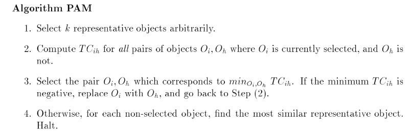
Take a look at the ch_05_kmedoids.R R code file from the bundle of R code for the previous algorithms. The code can be tested with the following command:
> source("ch_05_kmedoids.R")
Along with the increase in the size and quantity of documents on the Internet, the efficient algorithms are always in urgent need to get usable summarization or distill the key information. The documents will in versatile formats, structured or unstructured. The tasks include summarization of a single document or multiple documents. More extended target to extract summarization from multimedia files. Other challenges include summarizing multilingual documents. Abstraction requires the tool support from KNLP for grammar and lexicons for analyses and generation. One possible process for the abstraction is illustrated as follows:

Many approaches are suggested for automatic abstraction of document text, such as automatic extraction, automatic abstraction based on understanding, information extraction, and automatic abstraction based on structures. Possible features to be adapted to design the summarization system include the sentence length cutoff, fixed-phrase, paragraph, thematic word, and uppercase word features.
Abstraction or summarization popularly has been defined as a process with two steps. An intermediate representation of some sort is retrieved by the extraction of important concepts from the source texts. Given the intermediate representation, the summary is generated.
For the first step of the summarization process, it can largely be treated as part of automatic indexing. Lexical chains to extract important concepts from a document are one possible solution. Lexical chains exploit the cohesion among an arbitrary number of related words, and they are calculated by grouping (chaining) sets of words that are semantically related.
The PAM algorithm
The PAM (Partitioning Around Medoids) algorithm is a partitional clustering algorithm. The summarized pseudocode for the PAM algorithm is as follows:
Take a look at the ch_05_kmedoids.R R code file from the bundle of R code for the previous algorithms. The code can be tested with the following command:
> source("ch_05_kmedoids.R")
Along with the increase in the size and quantity of documents on the Internet, the efficient algorithms are always in urgent need to get usable summarization or distill the key information. The documents will in versatile formats, structured or unstructured. The tasks include summarization of a single document or multiple documents. More extended target to extract summarization from multimedia files. Other challenges include summarizing multilingual documents. Abstraction requires the tool support from KNLP for grammar and lexicons for analyses and generation. One possible process for the abstraction is illustrated as follows:
Many approaches are suggested for automatic abstraction of document text, such as automatic extraction, automatic abstraction based on understanding, information extraction, and automatic abstraction based on structures. Possible features to be adapted to design the summarization system include the sentence length cutoff, fixed-phrase, paragraph, thematic word, and uppercase word features.
Abstraction or summarization popularly has been defined as a process with two steps. An intermediate representation of some sort is retrieved by the extraction of important concepts from the source texts. Given the intermediate representation, the summary is generated.
For the first step of the summarization process, it can largely be treated as part of automatic indexing. Lexical chains to extract important concepts from a document are one possible solution. Lexical chains exploit the cohesion among an arbitrary number of related words, and they are calculated by grouping (chaining) sets of words that are semantically related.
The R implementation
Take a look at the ch_05_kmedoids.R R code file from the bundle of R code for the previous algorithms. The code can be tested with the following command:
> source("ch_05_kmedoids.R")
Along with the increase in the size and quantity of documents on the Internet, the efficient algorithms are always in urgent need to get usable summarization or distill the key information. The documents will in versatile formats, structured or unstructured. The tasks include summarization of a single document or multiple documents. More extended target to extract summarization from multimedia files. Other challenges include summarizing multilingual documents. Abstraction requires the tool support from KNLP for grammar and lexicons for analyses and generation. One possible process for the abstraction is illustrated as follows:
Many approaches are suggested for automatic abstraction of document text, such as automatic extraction, automatic abstraction based on understanding, information extraction, and automatic abstraction based on structures. Possible features to be adapted to design the summarization system include the sentence length cutoff, fixed-phrase, paragraph, thematic word, and uppercase word features.
Abstraction or summarization popularly has been defined as a process with two steps. An intermediate representation of some sort is retrieved by the extraction of important concepts from the source texts. Given the intermediate representation, the summary is generated.
For the first step of the summarization process, it can largely be treated as part of automatic indexing. Lexical chains to extract important concepts from a document are one possible solution. Lexical chains exploit the cohesion among an arbitrary number of related words, and they are calculated by grouping (chaining) sets of words that are semantically related.
Automatic abstraction and summarization of document text
Along with the increase in the size and quantity of documents on the Internet, the efficient algorithms are always in urgent need to get usable summarization or distill the key information. The documents will in versatile formats, structured or unstructured. The tasks include summarization of a single document or multiple documents. More extended target to extract summarization from multimedia files. Other challenges include summarizing multilingual documents. Abstraction requires the tool support from KNLP for grammar and lexicons for analyses and generation. One possible process for the abstraction is illustrated as follows:
Many approaches are suggested for automatic abstraction of document text, such as automatic extraction, automatic abstraction based on understanding, information extraction, and automatic abstraction based on structures. Possible features to be adapted to design the summarization system include the sentence length cutoff, fixed-phrase, paragraph, thematic word, and uppercase word features.
Abstraction or summarization popularly has been defined as a process with two steps. An intermediate representation of some sort is retrieved by the extraction of important concepts from the source texts. Given the intermediate representation, the summary is generated.
For the first step of the summarization process, it can largely be treated as part of automatic indexing. Lexical chains to extract important concepts from a document are one possible solution. Lexical chains exploit the cohesion among an arbitrary number of related words, and they are calculated by grouping (chaining) sets of words that are semantically related.
Instead of taking the whole set of data into consideration, the CLARA (Clustering LARge Application) algorithm randomly chooses a small portion of the actual data as a representative of the data. Medoids are then chosen from this sample using PAM. If the sample is selected in a fairly random manner, it should closely represent the original dataset.
CLARA draws multiple samples of the dataset, applies PAM to each sample, finds the medoids, and then returns its best clustering as the output. At first, a sample dataset D' is drawn from the original dataset D, and the PAM algorithm is applied to D' to find the k medoids. Use these k medoids and the dataset D to calculate the current dissimilarity. If it is smaller than the one you get in the previous iteration, then these k medoids are kept as the best k medoids. The whole process is performed a specified number of times.

CLARANS (Clustering Large Applications based on RANdomized Search) is efficient and effective and is the best practice for spatial data mining. CLARANS applies a strategy to search in a certain graph. A node in this graph, denoting it as  , is represented by a set of objects,
  ,
, . Here, k is the predefined value to choose the k medoids; as a result, the nodes in the graph are a set of
  . If two nodes,
  , and
, and  are neighbors, then
  . Each node in the graph represents a set of medoids and the cluster related to it. As a result, a cost is related to each node; this cost is the total distance between any objects and the medoid represents its cluster. The cost differential of two neighbors can be calculated with the cost measure function introduced in the PAM algorithm.

AP (Affinity Propagation) finds a set of exemplars,  , in the dataset and assigns nonselected points to the exemplars. An exemplar is the representative of a cluster.
Two types of messages are exchanged between data objects or points; they are explained here:
-
The r(i,k) message, which is called responsibility, represents the accumulated evidence sent from
 to
to  . It informs us that is suitable to serve as the exemplar of point . Every candidate is counted in.
-
The a(i,k) message, which is called availability, denotes the accumulated evidence sent from to . It informs us that should be the exemplar. Every support from other points is well considered.
Both r(i, k) and a(i,k) are initialized as 0 at the beginning of the algorithm:


 , for
, for s(k, k) is initialized with the same value (typically defined with heuristic knowledge) for each point at the start and updated in the following description to recur the affection. s(i, k) denotes the extent to which  is suited to be the exemplar of . Here is a possible value for
 s(i, i) to be set as a constant:


The index of exemplar,  , which is for data point
  , is defined with the following formula:
arg max {a(i,k) + r(i,k), k = 1,…, N}Given R = (r(i, j)) as the responsibility matrix and A = (a(i, j)) as the availability matrix, t represents the iteration counts, where a damping factor  is set to depress numerical oscillations that might arise:


Take a look at the ch_05_affinity_clustering.R R code file from the bundle of R code for the previously mentioned algorithms. The codes can be tested with the following command:
> source("ch_05_affinity_clustering.R")
Due to the massive number of images and other multimedia documents, the task to classify images becomes even harder than before. Unsupervised image categorization is frequently utilized by image and video summarization, or it just serves as a preprocessing step in supervised methods for classification.
One major issue related to unsupervised image categorization is to estimate the distribution of image categories. Further on, finding the most descriptive prototypes of the image categories is another main issue of image categorization.
Each image can be represented as a high-dimensional data instance, including features related to color, texture, and shape. The exemplar technique is applied here; it represents image categories by a small set of image or its fragments. Given exemplar concepts, the dimension of an image data instance reduces to a relatively small size and eases further processing. The measures applied here include the Chamfer, Hausdorff, and shuffle distances.
Natural categories of the dataset can be of various complex types; overlapping might be a frequent shape.
Unsupervised image categorization or classification is a clustering problem. Image clustering is to identify a set of similar image primitives, such as pixels, line elements, regions, and so on. Given the complex dataset, the recommended way is to use the prototype-based clustering algorithm. Affinity propagation algorithms can be applied to unsupervised categorization by finding a subset of representative exemplars.

Affinity propagation clustering
Affinity propagation itself is summarized as follows:

Take a look at the ch_05_affinity_clustering.R R code file from the bundle of R code for the previously mentioned algorithms. The codes can be tested with the following command:
> source("ch_05_affinity_clustering.R")
Due to the massive number of images and other multimedia documents, the task to classify images becomes even harder than before. Unsupervised image categorization is frequently utilized by image and video summarization, or it just serves as a preprocessing step in supervised methods for classification.
One major issue related to unsupervised image categorization is to estimate the distribution of image categories. Further on, finding the most descriptive prototypes of the image categories is another main issue of image categorization.
Each image can be represented as a high-dimensional data instance, including features related to color, texture, and shape. The exemplar technique is applied here; it represents image categories by a small set of image or its fragments. Given exemplar concepts, the dimension of an image data instance reduces to a relatively small size and eases further processing. The measures applied here include the Chamfer, Hausdorff, and shuffle distances.
Natural categories of the dataset can be of various complex types; overlapping might be a frequent shape.
Unsupervised image categorization or classification is a clustering problem. Image clustering is to identify a set of similar image primitives, such as pixels, line elements, regions, and so on. Given the complex dataset, the recommended way is to use the prototype-based clustering algorithm. Affinity propagation algorithms can be applied to unsupervised categorization by finding a subset of representative exemplars.
The R implementation
Take a look at the ch_05_affinity_clustering.R R code file from the bundle of R code for the previously mentioned algorithms. The codes can be tested with the following command:
> source("ch_05_affinity_clustering.R")
Due to the massive number of images and other multimedia documents, the task to classify images becomes even harder than before. Unsupervised image categorization is frequently utilized by image and video summarization, or it just serves as a preprocessing step in supervised methods for classification.
One major issue related to unsupervised image categorization is to estimate the distribution of image categories. Further on, finding the most descriptive prototypes of the image categories is another main issue of image categorization.
Each image can be represented as a high-dimensional data instance, including features related to color, texture, and shape. The exemplar technique is applied here; it represents image categories by a small set of image or its fragments. Given exemplar concepts, the dimension of an image data instance reduces to a relatively small size and eases further processing. The measures applied here include the Chamfer, Hausdorff, and shuffle distances.
Natural categories of the dataset can be of various complex types; overlapping might be a frequent shape.
Unsupervised image categorization or classification is a clustering problem. Image clustering is to identify a set of similar image primitives, such as pixels, line elements, regions, and so on. Given the complex dataset, the recommended way is to use the prototype-based clustering algorithm. Affinity propagation algorithms can be applied to unsupervised categorization by finding a subset of representative exemplars.
Unsupervised image categorization
Due to the massive number of images and other multimedia documents, the task to classify images becomes even harder than before. Unsupervised image categorization is frequently utilized by image and video summarization, or it just serves as a preprocessing step in supervised methods for classification.
One major issue related to unsupervised image categorization is to estimate the distribution of image categories. Further on, finding the most descriptive prototypes of the image categories is another main issue of image categorization.
Each image can be represented as a high-dimensional data instance, including features related to color, texture, and shape. The exemplar technique is applied here; it represents image categories by a small set of image or its fragments. Given exemplar concepts, the dimension of an image data instance reduces to a relatively small size and eases further processing. The measures applied here include the Chamfer, Hausdorff, and shuffle distances.
Natural categories of the dataset can be of various complex types; overlapping might be a frequent shape.
Unsupervised image categorization or classification is a clustering problem. Image clustering is to identify a set of similar image primitives, such as pixels, line elements, regions, and so on. Given the complex dataset, the recommended way is to use the prototype-based clustering algorithm. Affinity propagation algorithms can be applied to unsupervised categorization by finding a subset of representative exemplars.
Hierarchical clustering divides the target dataset into multilevels or a hierarchy of clusters. It segments data points along with successive partitions.
There are two strategies for hierarchical clustering. Agglomerative clustering starts with each data object in the input dataset as a cluster, and then in the following steps, clusters are merged according to certain similarity measures that end in only one cluster. Divisive clustering, in contrast, starts with one cluster with all the data objects in the input dataset as members, and then, the cluster splits according to certain similarity measures in the following steps, and at the end, singleton clusters of individual data objects are left.
The characteristics of hierarchical clustering methods are as follows:
- Multilevel decomposition.
- The merges or splits cannot perform a rollback. The error in the algorithm that is introduced by merging or splitting cannot be corrected.
- The hybrid algorithm.
The BIRCH (Balanced Iterative Reducing and Clustering using Hierarchies) algorithm is designed for large dynamic datasets and can also be applied to incremental and dynamic clustering. Only one pass of dataset is required, and this means that there is no need to read the whole dataset in advance.
CF-Tree
is a helper data structure that is used to store the summary of clusters, and it is also a representative of a cluster. Each node in the CF-Tree is declared as a list of entries,  , and
, and B is the predefined entry limitation.  denotes the link to the ith child.
Given  as the representative of cluster i, is defined as
  , where
  is the member count of the cluster, LS is the linear sum of the member objects, and SS is the squared sum of the member objects.
The leave of the CF-Tree must conform to the diameter limitation. The diameter of the  cluster must be less than the predefined threshold value, T.
The main helper algorithms in BIRCH are CF-Tree insertion and CF-Tree rebuilding.
The summarized pseudocode for the BIRCH algorithm is as follows:

The overall framework for the chameleon algorithm is illustrated in the following diagram:

There are three main steps in the chameleon algorithm, which are as follows:
- Sparsification: This step is to generate a k-Nearest Neighbor graph, which is derived from a proximity graph.
- Graph partitioning: This step applies a multilevel graph-partitioning algorithm to partition the dataset. The initial graph is an all-inclusive graph or cluster. This then bisects the largest graph in each successive step, and finally, we get a group of roughly, equally-sized clusters (with high intrasimilarity). Each resulting cluster has a size not more than a predefined size, that is,
MIN_SIZE. - Agglomerative hierarchical clustering: This last step is where the clusters are merged based on self-similarity. The notion of self-similarity is defined with the RI and RC; they can be combined in various ways to be a measure of self-similarity.
Relative Closeness (RC), given the  and
and  clusters with sizes
  and
and  , respectively.
  denotes the average weight of the edges that connect the two clusters.
  denotes the average weight of the edges that bisect the
  cluster:

Relative Interconnectivity (RI) is defined in the following equation. Here,  is the sum of the edges to connect the two clusters, and is the minimum sum of the cut edges that bisect the cluster:

The summarized pseudocode for the chameleon algorithm is as follows:

The probabilistic hierarchical clustering algorithm is a hybrid of hierarchical clustering and probabilistic clustering algorithms. As a probabilistic clustering algorithm, it applies a completely probabilistic approach, as depicted here:

Take a look at the ch_05_ahclustering.R R code file from the bundle of R code for the previously mentioned algorithms. The codes can be tested with the following command:
> source("ch_05_ahclustering.R")
News portals provide visitors with tremendous news categorized with a predefined set of topics. With the exponential growth of information we receive from the Internet, clustering technologies are widely used for web documents categorization, which include online news. These are often news streams or news feeds.
One advantage of a clustering algorithm for this task is that there is no need for prior domain knowledge. News can be summarized by clustering news that covers specific events. Unsupervised clustering can also play a pivotal role in discovering the intrinsic topical structure of the existing text collections, while new categorization is used to classify the documents according to a predefined set of classes.
Services such as Google News are provided. For a story published by a couple of new agencies or even the same agency, there are often various versions that exist at the same time or span the same range of days. Here, clustering can help aggregate the news related to the same story, and the result is a better overview of the current story for visitors.
As preprocessing steps, plain texts are extracted from the web pages or news pages. Reuters-22173 and -21578 are two popular documents dataset used for research. The representation of a data instance in the dataset can either be classical term-document vectors or term-sentence vectors, as the dataset is a collection of documents, and the cosine-like measures are applied here.
Agglomerative hierarchical clustering
The summarized pseudocode for the agglomerative hierarchical clustering algorithm is as follows:

The BIRCH (Balanced Iterative Reducing and Clustering using Hierarchies) algorithm is designed for large dynamic datasets and can also be applied to incremental and dynamic clustering. Only one pass of dataset is required, and this means that there is no need to read the whole dataset in advance.
CF-Tree
is a helper data structure that is used to store the summary of clusters, and it is also a representative of a cluster. Each node in the CF-Tree is declared as a list of entries, , and B is the predefined entry limitation. denotes the link to the ith child.
Given as the representative of cluster i, is defined as , where is the member count of the cluster, LS is the linear sum of the member objects, and SS is the squared sum of the member objects.
The leave of the CF-Tree must conform to the diameter limitation. The diameter of the cluster must be less than the predefined threshold value, T.
The main helper algorithms in BIRCH are CF-Tree insertion and CF-Tree rebuilding.
The summarized pseudocode for the BIRCH algorithm is as follows:
The overall framework for the chameleon algorithm is illustrated in the following diagram:
There are three main steps in the chameleon algorithm, which are as follows:
- Sparsification: This step is to generate a k-Nearest Neighbor graph, which is derived from a proximity graph.
- Graph partitioning: This step applies a multilevel graph-partitioning algorithm to partition the dataset. The initial graph is an all-inclusive graph or cluster. This then bisects the largest graph in each successive step, and finally, we get a group of roughly, equally-sized clusters (with high intrasimilarity). Each resulting cluster has a size not more than a predefined size, that is,
MIN_SIZE. - Agglomerative hierarchical clustering: This last step is where the clusters are merged based on self-similarity. The notion of self-similarity is defined with the RI and RC; they can be combined in various ways to be a measure of self-similarity.
Relative Closeness (RC), given the and clusters with sizes and , respectively. denotes the average weight of the edges that connect the two clusters. denotes the average weight of the edges that bisect the cluster:
Relative Interconnectivity (RI) is defined in the following equation. Here, is the sum of the edges to connect the two clusters, and is the minimum sum of the cut edges that bisect the cluster:
The summarized pseudocode for the chameleon algorithm is as follows:
The probabilistic hierarchical clustering algorithm is a hybrid of hierarchical clustering and probabilistic clustering algorithms. As a probabilistic clustering algorithm, it applies a completely probabilistic approach, as depicted here:
Take a look at the ch_05_ahclustering.R R code file from the bundle of R code for the previously mentioned algorithms. The codes can be tested with the following command:
> source("ch_05_ahclustering.R")
News portals provide visitors with tremendous news categorized with a predefined set of topics. With the exponential growth of information we receive from the Internet, clustering technologies are widely used for web documents categorization, which include online news. These are often news streams or news feeds.
One advantage of a clustering algorithm for this task is that there is no need for prior domain knowledge. News can be summarized by clustering news that covers specific events. Unsupervised clustering can also play a pivotal role in discovering the intrinsic topical structure of the existing text collections, while new categorization is used to classify the documents according to a predefined set of classes.
Services such as Google News are provided. For a story published by a couple of new agencies or even the same agency, there are often various versions that exist at the same time or span the same range of days. Here, clustering can help aggregate the news related to the same story, and the result is a better overview of the current story for visitors.
As preprocessing steps, plain texts are extracted from the web pages or news pages. Reuters-22173 and -21578 are two popular documents dataset used for research. The representation of a data instance in the dataset can either be classical term-document vectors or term-sentence vectors, as the dataset is a collection of documents, and the cosine-like measures are applied here.
The BIRCH algorithm
The BIRCH (Balanced Iterative Reducing and Clustering using Hierarchies) algorithm is designed for large dynamic datasets and can also be applied to incremental and dynamic clustering. Only one pass of dataset is required, and this means that there is no need to read the whole dataset in advance.
CF-Tree
is a helper data structure that is used to store the summary of clusters, and it is also a representative of a cluster. Each node in the CF-Tree is declared as a list of entries, , and B is the predefined entry limitation. denotes the link to the ith child.
Given as the representative of cluster i, is defined as , where is the member count of the cluster, LS is the linear sum of the member objects, and SS is the squared sum of the member objects.
The leave of the CF-Tree must conform to the diameter limitation. The diameter of the cluster must be less than the predefined threshold value, T.
The main helper algorithms in BIRCH are CF-Tree insertion and CF-Tree rebuilding.
The summarized pseudocode for the BIRCH algorithm is as follows:
The overall framework for the chameleon algorithm is illustrated in the following diagram:
There are three main steps in the chameleon algorithm, which are as follows:
- Sparsification: This step is to generate a k-Nearest Neighbor graph, which is derived from a proximity graph.
- Graph partitioning: This step applies a multilevel graph-partitioning algorithm to partition the dataset. The initial graph is an all-inclusive graph or cluster. This then bisects the largest graph in each successive step, and finally, we get a group of roughly, equally-sized clusters (with high intrasimilarity). Each resulting cluster has a size not more than a predefined size, that is,
MIN_SIZE. - Agglomerative hierarchical clustering: This last step is where the clusters are merged based on self-similarity. The notion of self-similarity is defined with the RI and RC; they can be combined in various ways to be a measure of self-similarity.
Relative Closeness (RC), given the and clusters with sizes and , respectively. denotes the average weight of the edges that connect the two clusters. denotes the average weight of the edges that bisect the cluster:
Relative Interconnectivity (RI) is defined in the following equation. Here, is the sum of the edges to connect the two clusters, and is the minimum sum of the cut edges that bisect the cluster:
The summarized pseudocode for the chameleon algorithm is as follows:
The probabilistic hierarchical clustering algorithm is a hybrid of hierarchical clustering and probabilistic clustering algorithms. As a probabilistic clustering algorithm, it applies a completely probabilistic approach, as depicted here:
Take a look at the ch_05_ahclustering.R R code file from the bundle of R code for the previously mentioned algorithms. The codes can be tested with the following command:
> source("ch_05_ahclustering.R")
News portals provide visitors with tremendous news categorized with a predefined set of topics. With the exponential growth of information we receive from the Internet, clustering technologies are widely used for web documents categorization, which include online news. These are often news streams or news feeds.
One advantage of a clustering algorithm for this task is that there is no need for prior domain knowledge. News can be summarized by clustering news that covers specific events. Unsupervised clustering can also play a pivotal role in discovering the intrinsic topical structure of the existing text collections, while new categorization is used to classify the documents according to a predefined set of classes.
Services such as Google News are provided. For a story published by a couple of new agencies or even the same agency, there are often various versions that exist at the same time or span the same range of days. Here, clustering can help aggregate the news related to the same story, and the result is a better overview of the current story for visitors.
As preprocessing steps, plain texts are extracted from the web pages or news pages. Reuters-22173 and -21578 are two popular documents dataset used for research. The representation of a data instance in the dataset can either be classical term-document vectors or term-sentence vectors, as the dataset is a collection of documents, and the cosine-like measures are applied here.
The chameleon algorithm
The overall framework for the chameleon algorithm is illustrated in the following diagram:
There are three main steps in the chameleon algorithm, which are as follows:
- Sparsification: This step is to generate a k-Nearest Neighbor graph, which is derived from a proximity graph.
- Graph partitioning: This step applies a multilevel graph-partitioning algorithm to partition the dataset. The initial graph is an all-inclusive graph or cluster. This then bisects the largest graph in each successive step, and finally, we get a group of roughly, equally-sized clusters (with high intrasimilarity). Each resulting cluster has a size not more than a predefined size, that is,
MIN_SIZE. - Agglomerative hierarchical clustering: This last step is where the clusters are merged based on self-similarity. The notion of self-similarity is defined with the RI and RC; they can be combined in various ways to be a measure of self-similarity.
Relative Closeness (RC), given the and clusters with sizes and , respectively. denotes the average weight of the edges that connect the two clusters. denotes the average weight of the edges that bisect the cluster:
Relative Interconnectivity (RI) is defined in the following equation. Here, is the sum of the edges to connect the two clusters, and is the minimum sum of the cut edges that bisect the cluster:
The summarized pseudocode for the chameleon algorithm is as follows:
The probabilistic hierarchical clustering algorithm is a hybrid of hierarchical clustering and probabilistic clustering algorithms. As a probabilistic clustering algorithm, it applies a completely probabilistic approach, as depicted here:
Take a look at the ch_05_ahclustering.R R code file from the bundle of R code for the previously mentioned algorithms. The codes can be tested with the following command:
> source("ch_05_ahclustering.R")
News portals provide visitors with tremendous news categorized with a predefined set of topics. With the exponential growth of information we receive from the Internet, clustering technologies are widely used for web documents categorization, which include online news. These are often news streams or news feeds.
One advantage of a clustering algorithm for this task is that there is no need for prior domain knowledge. News can be summarized by clustering news that covers specific events. Unsupervised clustering can also play a pivotal role in discovering the intrinsic topical structure of the existing text collections, while new categorization is used to classify the documents according to a predefined set of classes.
Services such as Google News are provided. For a story published by a couple of new agencies or even the same agency, there are often various versions that exist at the same time or span the same range of days. Here, clustering can help aggregate the news related to the same story, and the result is a better overview of the current story for visitors.
As preprocessing steps, plain texts are extracted from the web pages or news pages. Reuters-22173 and -21578 are two popular documents dataset used for research. The representation of a data instance in the dataset can either be classical term-document vectors or term-sentence vectors, as the dataset is a collection of documents, and the cosine-like measures are applied here.
The Bayesian hierarchical clustering algorithm
The summarized pseudocode for the Bayesian hierarchical clustering algorithm is as follows:

The probabilistic hierarchical clustering algorithm is a hybrid of hierarchical clustering and probabilistic clustering algorithms. As a probabilistic clustering algorithm, it applies a completely probabilistic approach, as depicted here:
Take a look at the ch_05_ahclustering.R R code file from the bundle of R code for the previously mentioned algorithms. The codes can be tested with the following command:
> source("ch_05_ahclustering.R")
News portals provide visitors with tremendous news categorized with a predefined set of topics. With the exponential growth of information we receive from the Internet, clustering technologies are widely used for web documents categorization, which include online news. These are often news streams or news feeds.
One advantage of a clustering algorithm for this task is that there is no need for prior domain knowledge. News can be summarized by clustering news that covers specific events. Unsupervised clustering can also play a pivotal role in discovering the intrinsic topical structure of the existing text collections, while new categorization is used to classify the documents according to a predefined set of classes.
Services such as Google News are provided. For a story published by a couple of new agencies or even the same agency, there are often various versions that exist at the same time or span the same range of days. Here, clustering can help aggregate the news related to the same story, and the result is a better overview of the current story for visitors.
As preprocessing steps, plain texts are extracted from the web pages or news pages. Reuters-22173 and -21578 are two popular documents dataset used for research. The representation of a data instance in the dataset can either be classical term-document vectors or term-sentence vectors, as the dataset is a collection of documents, and the cosine-like measures are applied here.
The probabilistic hierarchical clustering algorithm
The probabilistic hierarchical clustering algorithm is a hybrid of hierarchical clustering and probabilistic clustering algorithms. As a probabilistic clustering algorithm, it applies a completely probabilistic approach, as depicted here:
Take a look at the ch_05_ahclustering.R R code file from the bundle of R code for the previously mentioned algorithms. The codes can be tested with the following command:
> source("ch_05_ahclustering.R")
News portals provide visitors with tremendous news categorized with a predefined set of topics. With the exponential growth of information we receive from the Internet, clustering technologies are widely used for web documents categorization, which include online news. These are often news streams or news feeds.
One advantage of a clustering algorithm for this task is that there is no need for prior domain knowledge. News can be summarized by clustering news that covers specific events. Unsupervised clustering can also play a pivotal role in discovering the intrinsic topical structure of the existing text collections, while new categorization is used to classify the documents according to a predefined set of classes.
Services such as Google News are provided. For a story published by a couple of new agencies or even the same agency, there are often various versions that exist at the same time or span the same range of days. Here, clustering can help aggregate the news related to the same story, and the result is a better overview of the current story for visitors.
As preprocessing steps, plain texts are extracted from the web pages or news pages. Reuters-22173 and -21578 are two popular documents dataset used for research. The representation of a data instance in the dataset can either be classical term-document vectors or term-sentence vectors, as the dataset is a collection of documents, and the cosine-like measures are applied here.
The R implementation
Take a look at the ch_05_ahclustering.R R code file from the bundle of R code for the previously mentioned algorithms. The codes can be tested with the following command:
> source("ch_05_ahclustering.R")
News portals provide visitors with tremendous news categorized with a predefined set of topics. With the exponential growth of information we receive from the Internet, clustering technologies are widely used for web documents categorization, which include online news. These are often news streams or news feeds.
One advantage of a clustering algorithm for this task is that there is no need for prior domain knowledge. News can be summarized by clustering news that covers specific events. Unsupervised clustering can also play a pivotal role in discovering the intrinsic topical structure of the existing text collections, while new categorization is used to classify the documents according to a predefined set of classes.
Services such as Google News are provided. For a story published by a couple of new agencies or even the same agency, there are often various versions that exist at the same time or span the same range of days. Here, clustering can help aggregate the news related to the same story, and the result is a better overview of the current story for visitors.
As preprocessing steps, plain texts are extracted from the web pages or news pages. Reuters-22173 and -21578 are two popular documents dataset used for research. The representation of a data instance in the dataset can either be classical term-document vectors or term-sentence vectors, as the dataset is a collection of documents, and the cosine-like measures are applied here.
News categorization
News portals provide visitors with tremendous news categorized with a predefined set of topics. With the exponential growth of information we receive from the Internet, clustering technologies are widely used for web documents categorization, which include online news. These are often news streams or news feeds.
One advantage of a clustering algorithm for this task is that there is no need for prior domain knowledge. News can be summarized by clustering news that covers specific events. Unsupervised clustering can also play a pivotal role in discovering the intrinsic topical structure of the existing text collections, while new categorization is used to classify the documents according to a predefined set of classes.
Services such as Google News are provided. For a story published by a couple of new agencies or even the same agency, there are often various versions that exist at the same time or span the same range of days. Here, clustering can help aggregate the news related to the same story, and the result is a better overview of the current story for visitors.
As preprocessing steps, plain texts are extracted from the web pages or news pages. Reuters-22173 and -21578 are two popular documents dataset used for research. The representation of a data instance in the dataset can either be classical term-document vectors or term-sentence vectors, as the dataset is a collection of documents, and the cosine-like measures are applied here.
Here are some practice questions for you to check whether you understood the concepts we covered in this chapter:
- What is the PAM clustering algorithm?
- What is the k-means algorithm?
- What is the k-medoids algorithm?
- What is the CLARA algorithm?
- What is the CLARANS algorithm?
In this chapter, we looked at:
- Partition-based clustering.
- The k-means algorithm is a partition-based clustering algorithm. The centroids of clusters are defined as a representative of each cluster. In k-means clustering, a set of n data points in a D-dimensional space and an integer k are given. The problem is to distribute a set of k points in the centers to minimize the SSE.
- The k-medoids algorithm is a partition-based clustering algorithm. The representatives of each resulting clusters are chosen from the dataset itself, that is, the data objects belong to it.
- CLARA depends on sampling. It draws a sample from the original dataset instead of the entire dataset. PAM is then applied to each sampling. Then, the best result is kept during all the iterations.
- CLARANS is a clustering algorithm based on randomized search.
- The affinity propagation clustering algorithm recursively passes affinity messages between objects or points and converges to exemplars adaptively.
- Spectral clustering is used to construct graph partitions based on eigenvectors of the adjacency matrix.
- Hierarchical clustering decomposes a dataset D into levels of nested clusters; this is represented by a dendrogram, a tree that iteratively splits the dataset D into smaller subsets. The process stops only after each subset consists of only one object.
The next chapter will cover more advanced topics related to clustering algorithms, density-based algorithms, grid-based algorithms, the EM algorithm, high-dimensional algorithms, constraint-based clustering algorithms, and so on.
In this chapter, you will learn how to implement the top algorithms for clusters with R. The evaluation/benchmark/measure tools are also provided.
In this chapter, we will cover the following topics:
- Customer categorization analysis of e-commerce and DBSCAN
- Clustering web pages and OPTICS
- Visitor analysis in the browser cache and DENCLUE
- Recommendation system and STING
- Web sentiment analysis and CLIQUE
- Opinion mining and WAVE CLUSTER
- User search intent and the EM algorithm
- Customer purchase data analysis and clustering high-dimensional data
- SNS and clustering graph and network data
By defining the density and density measures of data point space, the clusters can be modeled as sections with certain density in the data space.
Density Based Spatial Clustering of Applications with Noise (DBSCAN) is one of the most popular density-based clustering algorithms. The major characteristics of DBSCAN are:
- Good at dealing with large datasets with noises
- Clusters of various shapes can be dealt with
DBSCAN is based on the classification of the data points in the dataset as core data points, border data points, and noise data points, with the support of the use of density relations between points, including directly density-reachable, density-reachable, density-connected points. Before we provide a detailed description of DBSCAN, let's illustrate these ideas.
A point is defined as a core point if the number of data points within the distance of the predefined parameter, Eps or  , is greater than that of the predefined parameter, MinPts. The space within the Eps is called Eps-neighborhood or
  . An object, o, is noise only if there is no cluster that contains o. A border data object is any object that belongs to a cluster, but not a core data object.
Given a core object, p, and an object, q, the object, q, is directly density-reachable from p if  .
.
Given a core object, p, and an object, q, the object q is density-reachable from p if  and
and  .
.
For two data objects,  and
and  , they are density-connected if
  .
.
The density-based cluster denotes a set of density-connected data objects that are maximal according to density reachability.
Here is an example illustrated in the following diagram:

The summarized pseudocode for the DBSCAN algorithm is as follows, with the following input/output parameters defined.
The input parameters for the DBSCAN algorithm are as follows:
- D, which is the training tuples dataset
- k, which is the neighbor list size
- Eps, which is the radius parameter that denotes the neighborhood area of a data point
- MinPts, which is the minimum number (the neighborhood density threshold) of points that must exist in the Eps-neighborhood
- The output of the algorithm
- A set of density-based clusters


Ordering points to identify the clustering structure, OPTICS, extends the DBSCAN algorithm and is based on the phenomenon that density-based clusters, with respect to a higher density, are completely contained in density-connected sets with respect to lower density.
To construct density-based clusters with different densities simultaneously, the objects are dealt with in a specific order when expanding a cluster, that is, according to the order, an object that is density-reachable with respect to the lowest for the higher density clusters will be finished first.
Two major concepts are introduced to illustrate the OPTICS algorithm: core-distance of an object, p, and reachability-distance of object, p. An example is illustrated in the following image. During which, core-distance (o), reachability-distances,  ,
, , for MinPts=4.

The core-distance of an object, p, is denoted as the minimal value,  , considering that the -neighborhood at least contains
 MinPts data objects; otherwise, this is undefined.
Given two data objects, p and q, the reachability-distance of object, p, from q represents the smallest radius value that makes p density-reachable from q if q is a core data object; otherwise, this is undefined.
OPTICS outputs an ordering of all data objects in a given dataset in which the data objects are processed. For each object, the core-distance and a suitable reachability-distance for each data object are calculated and output together.
OPTICS randomly selects an object from the input dataset as the current data object, p. In addition, for the object, p, the -neighborhood is fetched, the core-distance is calculated, and the reachability-distance is undefined.
Given p as a core data object, OPTICS recalculates the reachability-distance for any object, q (in the neighborhood of p), from p and inserts q into OrderSeeds if q has not been processed.
Once the augmented cluster ordering of the input dataset is generated with respect to , MinPts and a clustering-distance  , the density-based clustering is performed with this order.
The summarized pseudocode for the OPTICS algorithm with a couple of supporter functions are as follows:


Please take a look at the R codes file ch_06_optics.R from the bundle of R codes for the previously mentioned algorithm. The codes can be tested with the following command:
> source("ch_06_optics.R")
Clustering web pages can be used to group related texts/articles and serve as the preprocessing steps for supervised learning. It enables automated categorization.
Web pages are versatile and have a different structure (well-formed or badly formed without structure) and contents.
The Yahoo! industry web page data (CMUWeb KBProject, 1998) is used as the test data here.
The OPTICS algorithm
OPTICS randomly selects an object from the input dataset as the current data object, p. In addition, for the object, p, the -neighborhood is fetched, the core-distance is calculated, and the reachability-distance is undefined.
Given p as a core data object, OPTICS recalculates the reachability-distance for any object, q (in the neighborhood of p), from p and inserts q into OrderSeeds if q has not been processed.
Once the augmented cluster ordering of the input dataset is generated with respect to , MinPts and a clustering-distance , the density-based clustering is performed with this order.
The summarized pseudocode for the OPTICS algorithm with a couple of supporter functions are as follows:
Please take a look at the R codes file ch_06_optics.R from the bundle of R codes for the previously mentioned algorithm. The codes can be tested with the following command:
> source("ch_06_optics.R")
Clustering web pages can be used to group related texts/articles and serve as the preprocessing steps for supervised learning. It enables automated categorization.
Web pages are versatile and have a different structure (well-formed or badly formed without structure) and contents.
The Yahoo! industry web page data (CMUWeb KBProject, 1998) is used as the test data here.
The R implementation
Please take a look at the R codes file ch_06_optics.R from the bundle of R codes for the previously mentioned algorithm. The codes can be tested with the following command:
> source("ch_06_optics.R")
Clustering web pages can be used to group related texts/articles and serve as the preprocessing steps for supervised learning. It enables automated categorization.
Web pages are versatile and have a different structure (well-formed or badly formed without structure) and contents.
The Yahoo! industry web page data (CMUWeb KBProject, 1998) is used as the test data here.
Clustering web pages
Clustering web pages can be used to group related texts/articles and serve as the preprocessing steps for supervised learning. It enables automated categorization.
Web pages are versatile and have a different structure (well-formed or badly formed without structure) and contents.
The Yahoo! industry web page data (CMUWeb KBProject, 1998) is used as the test data here.
DENsity-based CLUstEring (DENCLUE) is a density-based clustering algorithm that depends on the support of density-distribution functions.
Before a detailed explanation on the DENCLUE algorithm, some concepts need to be introduced; they are influence function, density function, gradient, and density attractor.
The influence function of a specific data object can be any function for which the Gaussian kernel is usually used as the kernel at the data point.
The density function at a point, x, is defined as the sum of the influence functions of all the data objects at this data point.
A point is defined as a density attractor if it is a local maximum of the density function and is computed as


A gradient of the density function is defined in the following equation, given the density function,  .
.

DENCLUE defines a density function for the data point space at first. All the local maxima data points are searched and found. Assign each data point to the nearest local maxima point to maximize the density related to it. Each group of data points bound with a local maxima point is defined as a cluster. As a postprocess, the cluster is discarded if its bound local maxima density is lower than the user-predefined value. The clusters are merged if there exists a path such that each point on the path has a higher density value than the user-predefined value.

Please take a look at the R codes file ch_06_denclue.R from the bundle of R codes for previously mentioned algorithm. The codes can be tested with the following command:
> source("ch_06_denclue.R")
The browser-cache analysis provides the website owner with the convenience that shows the best matched part to the visitors, and at the same time, it is related to their privacy protection. The data instances in this context are browser caches, sessions, cookies, various logs, and so on.
The possible factors included in certain data instances can be the Web address, IP address (denotes the position where the visitor comes from), the duration for which the visitor stayed on a specific page, the pages the user visited, the sequence of the visited pages, the date and time of every visit, and so on. The log can be specific to a certain website or to various websites. A more detailed description is given in the following table:
The analysis of a visitor is basically history sniffing, which is used for user-behavior analysis.
The R implementation
Please take a look at the R codes file ch_06_denclue.R from the bundle of R codes for previously mentioned algorithm. The codes can be tested with the following command:
> source("ch_06_denclue.R")
The browser-cache analysis provides the website owner with the convenience that shows the best matched part to the visitors, and at the same time, it is related to their privacy protection. The data instances in this context are browser caches, sessions, cookies, various logs, and so on.
The possible factors included in certain data instances can be the Web address, IP address (denotes the position where the visitor comes from), the duration for which the visitor stayed on a specific page, the pages the user visited, the sequence of the visited pages, the date and time of every visit, and so on. The log can be specific to a certain website or to various websites. A more detailed description is given in the following table:
The analysis of a visitor is basically history sniffing, which is used for user-behavior analysis.
Visitor analysis in the browser cache
The browser-cache analysis provides the website owner with the convenience that shows the best matched part to the visitors, and at the same time, it is related to their privacy protection. The data instances in this context are browser caches, sessions, cookies, various logs, and so on.
The possible factors included in certain data instances can be the Web address, IP address (denotes the position where the visitor comes from), the duration for which the visitor stayed on a specific page, the pages the user visited, the sequence of the visited pages, the date and time of every visit, and so on. The log can be specific to a certain website or to various websites. A more detailed description is given in the following table:
The analysis of a visitor is basically history sniffing, which is used for user-behavior analysis.
STatistical Information Grid (STING) is a grid-based clustering algorithm. The dataset is recursively divided into a hierarchy structure. The whole input dataset serves as the root node in the hierarchy structure. Each cell/unit in a layer is composed of a couple of cells/units in the lower layer. An example is shown in the following diagram:

To support the query for a dataset, the statistical information of each unit is calculated in advance for further processing; this information is also called statistics parameters.
The characteristics of STING algorithms are (but not limited to) the following:
- A query-independent structure
- Intrinsically parallelizable
- Efficiency

Please take a look at the R codes file ch_06_sting.R from the bundle of R codes for the previously mentioned algorithm. The codes can be tested with the following command:
> source("ch_06_sting.R")
Depending on statistical, data-mining, and knowledge-discovery techniques, recommendation systems are being used by most of the e-commerce sites to make it easy for consumers to find products to purchase. Three main parts: representation of input data, neighborhood formation, and recommendation generation are shown in the following diagram:
The R implementation
Please take a look at the R codes file ch_06_sting.R from the bundle of R codes for the previously mentioned algorithm. The codes can be tested with the following command:
> source("ch_06_sting.R")
Depending on statistical, data-mining, and knowledge-discovery techniques, recommendation systems are being used by most of the e-commerce sites to make it easy for consumers to find products to purchase. Three main parts: representation of input data, neighborhood formation, and recommendation generation are shown in the following diagram:
Recommendation systems
Depending on statistical, data-mining, and knowledge-discovery techniques, recommendation systems are being used by most of the e-commerce sites to make it easy for consumers to find products to purchase. Three main parts: representation of input data, neighborhood formation, and recommendation generation are shown in the following diagram:
CLustering In QUEst (CLIQUE) is a bottom-up and grid-based clustering algorithm. The idea behind this algorithm is the Apriori feature, that is, the monotonicity of dense units with respect to dimensionality. If a set of data points, S, is a cluster in a k-dimensional projection of the space, then S is also contained in a cluster in any (k-1)-dimensional projections of this space.
The algorithm proceeds by passes. The one-dimensional dense units are produced by one pass through the data. The candidate k-dimensional units are generated using the candidate-generation procedure and the determined (k-l)-dimensional dense units that are fetched at the (k-1) pass.
The characteristics of the CLIQUE algorithm are as follows:
- Efficient for high-dimensional datasets
- Interpretability of results
- Scalability and usability
The CLIQUE algorithm contains three steps to cluster a dataset. First, a group of subspaces is selected to cluster the dataset. Then, clustering is independently executed in every subspace. Finally, a concise summary of every cluster is produced in the form of a disjunctive normal form (DNF) expression.
The summarized pseudocode for the CLIQUE algorithm is as follows:
- Indentification of subspaces that contain clusters.
- Indentification of cluster.
- Generation minimal description for the cluster.
The candidate-generation algorithm is illustrated as follows:

Here is the algorithm to find the connected components of the graph; this is equivalent to finding clusters:

Please take a look at the R codes file ch_06_clique.R from the bundle of R codes for the previously mentioned algorithm. The codes can be tested with the following command:
> source("ch_06_clique.R")
Web sentiment analysis is used to identify the idea or thought behind the text, for example, the sentiment analysis of microblogs such as Twitter. One simple example is comparing the post with a predefined labeled word list for sentiment judging. Another example is that we can judge a movie review as thumbs up or thumbs down.
Web sentiment analyses are used in news article analyses of biases pertaining to specific views, newsgroup evaluation, and so on.
The CLIQUE algorithm
The summarized pseudocode for the CLIQUE algorithm is as follows:
- Indentification of subspaces that contain clusters.
- Indentification of cluster.
- Generation minimal description for the cluster.
The candidate-generation algorithm is illustrated as follows:
Here is the algorithm to find the connected components of the graph; this is equivalent to finding clusters:
Please take a look at the R codes file ch_06_clique.R from the bundle of R codes for the previously mentioned algorithm. The codes can be tested with the following command:
> source("ch_06_clique.R")
Web sentiment analysis is used to identify the idea or thought behind the text, for example, the sentiment analysis of microblogs such as Twitter. One simple example is comparing the post with a predefined labeled word list for sentiment judging. Another example is that we can judge a movie review as thumbs up or thumbs down.
Web sentiment analyses are used in news article analyses of biases pertaining to specific views, newsgroup evaluation, and so on.
The R implementation
Please take a look at the R codes file ch_06_clique.R from the bundle of R codes for the previously mentioned algorithm. The codes can be tested with the following command:
> source("ch_06_clique.R")
Web sentiment analysis is used to identify the idea or thought behind the text, for example, the sentiment analysis of microblogs such as Twitter. One simple example is comparing the post with a predefined labeled word list for sentiment judging. Another example is that we can judge a movie review as thumbs up or thumbs down.
Web sentiment analyses are used in news article analyses of biases pertaining to specific views, newsgroup evaluation, and so on.
Web sentiment analysis
Web sentiment analysis is used to identify the idea or thought behind the text, for example, the sentiment analysis of microblogs such as Twitter. One simple example is comparing the post with a predefined labeled word list for sentiment judging. Another example is that we can judge a movie review as thumbs up or thumbs down.
Web sentiment analyses are used in news article analyses of biases pertaining to specific views, newsgroup evaluation, and so on.
The WAVE clustering algorithm is a grid-based clustering algorithm. It depends on the relation between spatial dataset and multidimensional signals. The idea is that the cluster in a multidimensional spatial dataset turns out to be more distinguishable after a wavelet transformation, that is, after applying wavelets to the input data or the preprocessed input dataset. The dense part segmented by the sparse area in the transformed result represents clusters.
The characteristics of the WAVE cluster algorithm are as follows:
- Efficient for a large dataset
- Efficient for finding various shapes of clusters
- Insensitive to noise or outlier
- Insensitive with respect to the input order of a dataset
- Multiresolution, which is introduced by wavelet transforms
- Applicable to any numerical dataset
The WAVE cluster algorithm performs a few steps. In the first step, it creates a grid and assigns each data object from the input dataset to a unit in the grid. And then, transform the data to a new space by applying wavelet transform functions. Third, find the connected component in the new space. Map the cluster label for related data object to the original data space.

Please take a look at the R codes file ch_06_wave.R from the bundle of R codes for the previously mentioned algorithm. The codes can be tested with the following command:
> source("ch_06_wave.R")
An entity possesses a couple of features. Features might be explicit or implicit. If a person or organization expresses an opinion, then the person or organization should be an opinion holder. An opinion specific to a feature is a positive or negative view, attitude, emotion, or appraisal of the feature from the opinion holder. Whether the opinion on a feature is positive, negative, or neutral denotes opinion orientation.
Opinion mining means mining the opinion on certain features of the object or entity under research. The simplest case is to judge the opinion as positive or negative.
An opinion-orientation algorithm can be listed as follows:
- Identify opinion words and phrases
- Handle negation
- The But clause
- Aggregating opinion

The preceding formula denotes the opinion orientation on a certain feature,  , where
  is an opinion word in s,
  is the distance between and .
  is the opinion orientation.
Please take a look at the R codes file ch_06_wave.R from the bundle of R codes for the previously mentioned algorithm. The codes can be tested with the following command:
> source("ch_06_wave.R")
An entity possesses a couple of features. Features might be explicit or implicit. If a person or organization expresses an opinion, then the person or organization should be an opinion holder. An opinion specific to a feature is a positive or negative view, attitude, emotion, or appraisal of the feature from the opinion holder. Whether the opinion on a feature is positive, negative, or neutral denotes opinion orientation.
Opinion mining means mining the opinion on certain features of the object or entity under research. The simplest case is to judge the opinion as positive or negative.
An opinion-orientation algorithm can be listed as follows:
- Identify opinion words and phrases
- Handle negation
- The But clause
- Aggregating opinion
The preceding formula denotes the opinion orientation on a certain feature, , where is an opinion word in s, is the distance between and . is the opinion orientation.
The R implementation
Please take a look at the R codes file ch_06_wave.R from the bundle of R codes for the previously mentioned algorithm. The codes can be tested with the following command:
> source("ch_06_wave.R")
An entity possesses a couple of features. Features might be explicit or implicit. If a person or organization expresses an opinion, then the person or organization should be an opinion holder. An opinion specific to a feature is a positive or negative view, attitude, emotion, or appraisal of the feature from the opinion holder. Whether the opinion on a feature is positive, negative, or neutral denotes opinion orientation.
Opinion mining means mining the opinion on certain features of the object or entity under research. The simplest case is to judge the opinion as positive or negative.
An opinion-orientation algorithm can be listed as follows:
- Identify opinion words and phrases
- Handle negation
- The But clause
- Aggregating opinion
The preceding formula denotes the opinion orientation on a certain feature, , where is an opinion word in s, is the distance between and . is the opinion orientation.
Opinion mining
An entity possesses a couple of features. Features might be explicit or implicit. If a person or organization expresses an opinion, then the person or organization should be an opinion holder. An opinion specific to a feature is a positive or negative view, attitude, emotion, or appraisal of the feature from the opinion holder. Whether the opinion on a feature is positive, negative, or neutral denotes opinion orientation.
Opinion mining means mining the opinion on certain features of the object or entity under research. The simplest case is to judge the opinion as positive or negative.
An opinion-orientation algorithm can be listed as follows:
- Identify opinion words and phrases
- Handle negation
- The But clause
- Aggregating opinion
The preceding formula denotes the opinion orientation on a certain feature, , where is an opinion word in s, is the distance between and . is the opinion orientation.
The Expectation Maximization (EM) algorithm is a probabilistic-model-based clustering algorithm that depends on the mixture model in which the data is modeled by a mixture of simple models. The parameters related to these models are estimated by Maximum Likelihood Estimation (MLE).
Mixture models assume that the data is the result of the combination of various simple probabilistic distribution functions. Given K distribution functions and the jth distribution with the parameter,  ,
,  is the set of of all distributions:

The EM algorithm performs in the following way. In the first step, an initial group of model parameters are selected. The expectation step is the second step that performs the calculation of the probability:

The previous equation represents the probability of each data object belonging to each distribution. Maximization is the third step. With the result of the expectation step, update the estimation of the parameters with the ones that maximize the expected likelihood:


The expectation step and maximization step are performed repeatedly until the output matches the ending condition, that is, the changes of the parameter estimations below a certain threshold.

Please take a look at the R codes file ch_06_em.R from the bundle of R codes for the previously mentioned algorithm. The codes can be tested with the following command:
> source("ch_06_em.R")
Determining the user search intent is an important yet a difficult issue with respect to the sparse data available concerning the searcher and queries.
User intent has a wide range of applications, cluster query refinements, user intention profiles, and web search intent induction. Given Web search engine queries, finding user intention is also a key and requirement.
To determine the user interest and preferences, the clicks' sequence upon the search result can be used as a good base.
Web search personalization is another important application with the user search intention. It is related to user context and intention. With the user intention applied, more effective and efficient information will be provided.
The R implementation
Please take a look at the R codes file ch_06_em.R from the bundle of R codes for the previously mentioned algorithm. The codes can be tested with the following command:
> source("ch_06_em.R")
Determining the user search intent is an important yet a difficult issue with respect to the sparse data available concerning the searcher and queries.
User intent has a wide range of applications, cluster query refinements, user intention profiles, and web search intent induction. Given Web search engine queries, finding user intention is also a key and requirement.
To determine the user interest and preferences, the clicks' sequence upon the search result can be used as a good base.
Web search personalization is another important application with the user search intention. It is related to user context and intention. With the user intention applied, more effective and efficient information will be provided.
The user search intent
Determining the user search intent is an important yet a difficult issue with respect to the sparse data available concerning the searcher and queries.
User intent has a wide range of applications, cluster query refinements, user intention profiles, and web search intent induction. Given Web search engine queries, finding user intention is also a key and requirement.
To determine the user interest and preferences, the clicks' sequence upon the search result can be used as a good base.
Web search personalization is another important application with the user search intention. It is related to user context and intention. With the user intention applied, more effective and efficient information will be provided.
For high-dimensional data-space clustering, two major issues occur: efficiency and quality. New algorithms are needed to deal with this type of dataset. Two popular strategies are applied to it. One is the subspace-clustering strategy to find the cluster in the subspace of the original dataset space. Another is the dimensionality-reduction strategy, which is a lower dimensional data space created for further clustering.
MAFIA is an efficient and scalable subspace-clustering algorithm for high-dimensional and large datasets.
The summarized pseudocode for the MAFIA algorithm is as follows:

The summarized pseudocode for the parallel MAFIA algorithm is as follows:

The summarized pseudocodes for the SURFING algorithm are as follows. It selects interesting features from the original attributes of the dataset.

The MAFIA algorithm
The summarized pseudocode for the MAFIA algorithm is as follows:
The summarized pseudocode for the parallel MAFIA algorithm is as follows:
The summarized pseudocodes for the SURFING algorithm are as follows. It selects interesting features from the original attributes of the dataset.
The SURFING algorithm
The summarized pseudocodes for the SURFING algorithm are as follows. It selects interesting features from the original attributes of the dataset.
The clustering for graph and network data has a wide application in modern life, such as social networking. However, more challenges crop up along with the needs. High computational cost, sophisticated graphs, and high dimensionality and sparsity are the major concerns. With some special transformations, the issues can be transformed into graph cut issues.
Structural Clustering Algorithm for Network (SCAN) is one of the algorithms that searches for well-connected components in the graph as clusters.


Please take a look at the R codes file ch_06_scan.R from the bundle of R codes for the previously mentioned algorithms. The codes can be tested with the following command:
> source("ch_06_scan.R")
Social network has become the most popular online communication method nowadays. The analysis of SNS becomes important, because of the requirement of security, business, control, and so on.
The foundation of SNS is a graph theory, especially for SNS mining, such as finding social communities and abuse of SNS for bad purpose.
The clustering for SNS is an inherent application to find a community (or community detection). Random walk is another key technology for SNS analysis and is used to find communities.
The R implementation
Please take a look at the R codes file ch_06_scan.R from the bundle of R codes for the previously mentioned algorithms. The codes can be tested with the following command:
> source("ch_06_scan.R")
Social network has become the most popular online communication method nowadays. The analysis of SNS becomes important, because of the requirement of security, business, control, and so on.
The foundation of SNS is a graph theory, especially for SNS mining, such as finding social communities and abuse of SNS for bad purpose.
The clustering for SNS is an inherent application to find a community (or community detection). Random walk is another key technology for SNS analysis and is used to find communities.
Social networking service (SNS)
Social network has become the most popular online communication method nowadays. The analysis of SNS becomes important, because of the requirement of security, business, control, and so on.
The foundation of SNS is a graph theory, especially for SNS mining, such as finding social communities and abuse of SNS for bad purpose.
The clustering for SNS is an inherent application to find a community (or community detection). Random walk is another key technology for SNS analysis and is used to find communities.
Here are some questions for you to know whether you have understood the concepts:
- What is the DBSCAN algorithm?
- What is the SCAN algorithm?
- What is the STING algorithm?
- What is the OPTICS algorithm?
- What is the constraint-based cluster method?
In this chapter, we covered the following facts:
- DBSCAN depends on the density-based description of clusters. With searching and measuring the density of data points, high density means high possibility of the existence of clusters, and others mean outliers or noise.
- OPTICS produces the cluster ordering that consists of the order of the data objects together with the corresponding reachability values and core values.
- You learned that DENCLUE is a clustering algorithm based on a set of specific density-distribution functions and can find arbitrary shape clusters. It first segments the dataset as cubes and identifies the local density-distribution function. You also learned that a hill-climbing algorithm is performed to retrieve the local maximum for each item in the related cube with which a cluster will be built.
- We saw that STING is based on the grid-like data structure, and it segments the embedding spatial area of the input data points into rectangular units. It is mainly used for a spatial dataset.
- You learned that CLIQUE is a grid-based clustering algorithm that finds subspaces of high-dimensional data, and it can find dense units in the high-dimensional data too.
- You know that the WAVE cluster is a grid-based clustering algorithm based on the wavelet transformations. It has a multiresolution and is efficient for large dataset.
- You learned that EM is a probabilistic-model-based clustering algorithm, where each data point with a probability indicates that it belongs to a cluster. It is based on the assumption that the attribute of the data point has values that is the linear combination of simple distributions.
- Clustering high-dimensional data.
- Clustering graph and network data.
In the next chapter, we will cover the major topics related to outlier detection and algorithms, and look at some of their examples.
In this chapter, you will learn how to write R codes to detect outliers in real-world cases. Generally speaking, outliers arise for various reasons, such as the dataset being compromised with data from different classes and data measurement system errors.
As per their characteristics, outliers differ dramatically from the usual data in the original dataset. Versatile solutions are developed to detect them, which include model-based methods, proximity-based methods, density-based methods, and so on.
In this chapter, we will cover the following topics:
- Credit card fraud detection and statistical methods
- Activity monitoring—the detection of fraud of mobile phones and proximity-based methods
- Intrusion detection and density-based methods
- Intrusion detection and clustering-based methods
- Monitoring the performance of network-based and classification-based methods
- Detecting novelty in text, topic detection, and mining contextual outliers
- Collective outliers on spatial data
- Outlier detection in high-dimensional data
Here is a diagram illustrating a classification of outlier detection methods:

The output of an outlier detection system can be categorized into two groups: one is the labeled result and the other is the scored result (or an ordered list).
One major solution to detect outliers is the model-based method or statistical method. The outlier is defined as the object not belonging to the model that is used to represent the original dataset. In other words, that model does not generate the outlier.
Among the accurate models to be adopted for the specific dataset, there are many choices available such as Gaussian and Poisson. If the wrong model is used to detect outliers, the normal data point may wrongly be recognized as an outlier. In addition to applying the single distribution model, the mixture of distribution models is practical too.

The log-likelihood function is adopted to find the estimation of parameters of a model:


Look up the file of R codes, ch_07_lboutlier_detection.R, from the bundle of R codes for the previously mentioned algorithm. The codes can be tested with the following command:
> source("ch_07_lboutlier_detection.R")
Fraud denotes the criminal activities that happen in various commercial companies, such as credit card, banking, or insurance companies. For credit card fraud detection, two major applications are covered, fraudulent application of credit card and fraudulent usage of credit card. The fraud represents behavior anomalous to the average usage of credit cards to certain users, that is, transaction records of the users.
This kind of outlier statistically denotes credit card theft, which deviates from the normal nature of criminal activities. Some examples of outliers in this case are high rate of purchase, very high payments, and so on.
The location of payment, the user, and the context are possible attributes in the dataset. The clustering algorithms are the possible solutions.
Two major approaches of proximity-based methods are distance-based and density-based outlier detection algorithms.


The summarized pseudocodes of the distance-based outlier detection algorithm are as follows, given a dataset D, size of the input dataset n, threshold r (r > 0), and  :
:

A  outlier is defined as a data point,
 o, and subjected to this formula:

Let's now learn the pseudocodes for a variety of distance-based outlier detection algorithms, which are summarized in the following list. The input parameters are k, n, and D, which represent the neighbors' number, outlier number to be identified, and input dataset, respectively. A few supporter functions also are defined. Nearest (o, S, k) returns k nearest objects in S to o, Maxdist (o, S) returns the maximum distance between o and points from S, and TopOutlier (S, n) returns the top n outliers in S according to the distance to their kth nearest neighbor.

The Dolphin algorithm is a distance-based outlier detection algorithm. The summarized pseudocodes of this algorithm are listed as follows:


Look up the file of R codes, ch_07_proximity_based.R, from the bundle of R codes for the preceding algorithms. The codes can be tested with the following command:
> source("ch_07_proximity_based.R")
The purpose of outlier detection is to find the patterns in source datasets that do not conform to the standard behavior. The dataset here consists of the calling records, and the patterns exist in the calling records.
There are many special algorithms developed for each specific domain. Misuse of a mobile is termed as mobile fraud. The subject under research is the calling activity or call records. The related attributes include, but are not limited to, call duration, calling city, call day, and various services' ratios.
The summarized pseudocodes of the distance-based outlier detection algorithm are as follows, given a dataset D, size of the input dataset n, threshold r (r > 0), and :
A outlier is defined as a data point, o, and subjected to this formula:
Let's now learn the pseudocodes for a variety of distance-based outlier detection algorithms, which are summarized in the following list. The input parameters are k, n, and D, which represent the neighbors' number, outlier number to be identified, and input dataset, respectively. A few supporter functions also are defined. Nearest (o, S, k) returns k nearest objects in S to o, Maxdist (o, S) returns the maximum distance between o and points from S, and TopOutlier (S, n) returns the top n outliers in S according to the distance to their kth nearest neighbor.
The Dolphin algorithm is a distance-based outlier detection algorithm. The summarized pseudocodes of this algorithm are listed as follows:
Look up the file of R codes, ch_07_proximity_based.R, from the bundle of R codes for the preceding algorithms. The codes can be tested with the following command:
> source("ch_07_proximity_based.R")
The purpose of outlier detection is to find the patterns in source datasets that do not conform to the standard behavior. The dataset here consists of the calling records, and the patterns exist in the calling records.
There are many special algorithms developed for each specific domain. Misuse of a mobile is termed as mobile fraud. The subject under research is the calling activity or call records. The related attributes include, but are not limited to, call duration, calling city, call day, and various services' ratios.
The FindAllOutsM algorithm
The following are the summarized pseudocode of the FindAllOutsM algorithm:

The summarized pseudocodes of the distance-based outlier detection algorithm are as follows, given a dataset D, size of the input dataset n, threshold r (r > 0), and :
A outlier is defined as a data point, o, and subjected to this formula:
Let's now learn the pseudocodes for a variety of distance-based outlier detection algorithms, which are summarized in the following list. The input parameters are k, n, and D, which represent the neighbors' number, outlier number to be identified, and input dataset, respectively. A few supporter functions also are defined. Nearest (o, S, k) returns k nearest objects in S to o, Maxdist (o, S) returns the maximum distance between o and points from S, and TopOutlier (S, n) returns the top n outliers in S according to the distance to their kth nearest neighbor.
The Dolphin algorithm is a distance-based outlier detection algorithm. The summarized pseudocodes of this algorithm are listed as follows:
Look up the file of R codes, ch_07_proximity_based.R, from the bundle of R codes for the preceding algorithms. The codes can be tested with the following command:
> source("ch_07_proximity_based.R")
The purpose of outlier detection is to find the patterns in source datasets that do not conform to the standard behavior. The dataset here consists of the calling records, and the patterns exist in the calling records.
There are many special algorithms developed for each specific domain. Misuse of a mobile is termed as mobile fraud. The subject under research is the calling activity or call records. The related attributes include, but are not limited to, call duration, calling city, call day, and various services' ratios.
The distance-based algorithm
The summarized pseudocodes of the distance-based outlier detection algorithm are as follows, given a dataset D, size of the input dataset n, threshold r (r > 0), and :
A outlier is defined as a data point, o, and subjected to this formula:
Let's now learn the pseudocodes for a variety of distance-based outlier detection algorithms, which are summarized in the following list. The input parameters are k, n, and D, which represent the neighbors' number, outlier number to be identified, and input dataset, respectively. A few supporter functions also are defined. Nearest (o, S, k) returns k nearest objects in S to o, Maxdist (o, S) returns the maximum distance between o and points from S, and TopOutlier (S, n) returns the top n outliers in S according to the distance to their kth nearest neighbor.
The Dolphin algorithm is a distance-based outlier detection algorithm. The summarized pseudocodes of this algorithm are listed as follows:
Look up the file of R codes, ch_07_proximity_based.R, from the bundle of R codes for the preceding algorithms. The codes can be tested with the following command:
> source("ch_07_proximity_based.R")
The purpose of outlier detection is to find the patterns in source datasets that do not conform to the standard behavior. The dataset here consists of the calling records, and the patterns exist in the calling records.
There are many special algorithms developed for each specific domain. Misuse of a mobile is termed as mobile fraud. The subject under research is the calling activity or call records. The related attributes include, but are not limited to, call duration, calling city, call day, and various services' ratios.
The Dolphin algorithm
The Dolphin algorithm is a distance-based outlier detection algorithm. The summarized pseudocodes of this algorithm are listed as follows:
Look up the file of R codes, ch_07_proximity_based.R, from the bundle of R codes for the preceding algorithms. The codes can be tested with the following command:
> source("ch_07_proximity_based.R")
The purpose of outlier detection is to find the patterns in source datasets that do not conform to the standard behavior. The dataset here consists of the calling records, and the patterns exist in the calling records.
There are many special algorithms developed for each specific domain. Misuse of a mobile is termed as mobile fraud. The subject under research is the calling activity or call records. The related attributes include, but are not limited to, call duration, calling city, call day, and various services' ratios.
The R implementation
Look up the file of R codes, ch_07_proximity_based.R, from the bundle of R codes for the preceding algorithms. The codes can be tested with the following command:
> source("ch_07_proximity_based.R")
The purpose of outlier detection is to find the patterns in source datasets that do not conform to the standard behavior. The dataset here consists of the calling records, and the patterns exist in the calling records.
There are many special algorithms developed for each specific domain. Misuse of a mobile is termed as mobile fraud. The subject under research is the calling activity or call records. The related attributes include, but are not limited to, call duration, calling city, call day, and various services' ratios.
Activity monitoring and the detection of mobile fraud
The purpose of outlier detection is to find the patterns in source datasets that do not conform to the standard behavior. The dataset here consists of the calling records, and the patterns exist in the calling records.
There are many special algorithms developed for each specific domain. Misuse of a mobile is termed as mobile fraud. The subject under research is the calling activity or call records. The related attributes include, but are not limited to, call duration, calling city, call day, and various services' ratios.
Here is a formal definition of outliers formalized based on concepts such as, LOF, LRD, and so on. Generally speaking, an outlier is a data point biased from others so much that it seems as if it has not been generated from the same distribution functions as others have been.
Given a dataset, D, a DB (x, y)-outlier, p, is defined like this:

The k-distance of the p data point denotes the distance between p and the data point, o, which is member of D:


The k-distance neighborhood of the p object is defined as follows, q being the k-Nearest Neighbor of p:

The following formula gives the reachability distance of an object, p, with respect to an object, o:

The Local Reachability Density (LRD) of a data object, o, is defined like this:

The Local Outlier Factor (LOF) is defined as follows, and it measures the degree of the outlierness:

A property of LOF (p) is defined as shown in the following equation:


These equations are illustrated as follows:

The input parameters for the bagging algorithm are:
 , the dataset
 , the parameter
 , another parameter
The output of the algorithm is the value of CBLOF, for all records.
The summarized pseudocodes of the OPTICS-OF algorithm are as follows:

The summarized pseudocodes of the High Contrast Subspace (HiCS) algorithm are as follows, where the input parameters are S, M, and  . The output is a contrast,
 |S|.

Look up the file of R codes, ch_07_ density _based.R, from the bundle of R codes for the previously mentioned algorithms. The codes can be tested using the following command:
> source("ch_07_ density _based.R")
Any malicious activity against systems, networks, and servers can be treated as intrusion, and finding such activities is called intrusion detection.
The characteristics of situations where you can detect intrusion are high volume of data, missing labeled data in the dataset (which can be training data for some specific solution), time series data, and false alarm rate in the input dataset.
An intrusion detection system is of two types: host-based and network-based intrusion detection systems. A popular architecture for intrusion detection based on data mining is illustrated in the following diagram:

The core algorithms applied in an outlier detection system are usually semi-supervised or unsupervised according to the characteristics of intrusion detection.
The OPTICS-OF algorithm
The input parameters for the bagging algorithm are:
- , the dataset
- , the parameter
- , another parameter
The output of the algorithm is the value of CBLOF, for all records.
The summarized pseudocodes of the OPTICS-OF algorithm are as follows:
The summarized pseudocodes of the High Contrast Subspace (HiCS) algorithm are as follows, where the input parameters are S, M, and . The output is a contrast, |S|.
Look up the file of R codes, ch_07_ density _based.R, from the bundle of R codes for the previously mentioned algorithms. The codes can be tested using the following command:
> source("ch_07_ density _based.R")
Any malicious activity against systems, networks, and servers can be treated as intrusion, and finding such activities is called intrusion detection.
The characteristics of situations where you can detect intrusion are high volume of data, missing labeled data in the dataset (which can be training data for some specific solution), time series data, and false alarm rate in the input dataset.
An intrusion detection system is of two types: host-based and network-based intrusion detection systems. A popular architecture for intrusion detection based on data mining is illustrated in the following diagram:
The core algorithms applied in an outlier detection system are usually semi-supervised or unsupervised according to the characteristics of intrusion detection.
The High Contrast Subspace algorithm
The summarized pseudocodes of the High Contrast Subspace (HiCS) algorithm are as follows, where the input parameters are S, M, and . The output is a contrast, |S|.
Look up the file of R codes, ch_07_ density _based.R, from the bundle of R codes for the previously mentioned algorithms. The codes can be tested using the following command:
> source("ch_07_ density _based.R")
Any malicious activity against systems, networks, and servers can be treated as intrusion, and finding such activities is called intrusion detection.
The characteristics of situations where you can detect intrusion are high volume of data, missing labeled data in the dataset (which can be training data for some specific solution), time series data, and false alarm rate in the input dataset.
An intrusion detection system is of two types: host-based and network-based intrusion detection systems. A popular architecture for intrusion detection based on data mining is illustrated in the following diagram:
The core algorithms applied in an outlier detection system are usually semi-supervised or unsupervised according to the characteristics of intrusion detection.
The R implementation
Look up the file of R codes, ch_07_ density _based.R, from the bundle of R codes for the previously mentioned algorithms. The codes can be tested using the following command:
> source("ch_07_ density _based.R")
Any malicious activity against systems, networks, and servers can be treated as intrusion, and finding such activities is called intrusion detection.
The characteristics of situations where you can detect intrusion are high volume of data, missing labeled data in the dataset (which can be training data for some specific solution), time series data, and false alarm rate in the input dataset.
An intrusion detection system is of two types: host-based and network-based intrusion detection systems. A popular architecture for intrusion detection based on data mining is illustrated in the following diagram:
The core algorithms applied in an outlier detection system are usually semi-supervised or unsupervised according to the characteristics of intrusion detection.
Intrusion detection
Any malicious activity against systems, networks, and servers can be treated as intrusion, and finding such activities is called intrusion detection.
The characteristics of situations where you can detect intrusion are high volume of data, missing labeled data in the dataset (which can be training data for some specific solution), time series data, and false alarm rate in the input dataset.
An intrusion detection system is of two types: host-based and network-based intrusion detection systems. A popular architecture for intrusion detection based on data mining is illustrated in the following diagram:
The core algorithms applied in an outlier detection system are usually semi-supervised or unsupervised according to the characteristics of intrusion detection.
The strategy of outlier detection technologies based on the clustering algorithm is focused on the relation between data objects and clusters.
Outlier detection that uses the hierarchical clustering algorithm is based on the k-Nearest Neighbor graph. The input parameters include the input dataset, DATA, of size, n, and each data point with k variables, the distance measure function (d), one hierarchical algorithm (h), threshold (t), and cluster number (nc).

The process of the outlier detection based on the k-means algorithm is illustrated in the following diagram:

The summarized pseudocodes of outlier detection using the k-means algorithm are as follows:
- Phase 1 (Data preparation):
- The target observations and attributes should be aligned to improve the accuracy of the result and performance of the k-means clustering algorithm.
- If the original dataset has missing data, its handling activity must be carried out. The data of maximum likelihood that is anticipated by the EM algorithm is fed as input into the missing data.
- Phase 2 (The outlier detection procedure):
- The k value should be determined in order to run the k-means clustering algorithm. The proper k value is decided by referring to the value of the Cubic Clustering Criterion.
- The k-means clustering algorithm runs with the decided k value. On completion, the expert checks the external and internal outliers in the clustering results. If the other groups' elimination of the outliers is more meaningful, then he/she stops this procedure. If the other groups need to be recalculated, he/she again runs the k-means clustering algorithms but without the detected outliers.
- Phase 3 (Review and validation):
- The result of the previous phase is only a candidate for this phase. By considering the domain knowledge, we can find the true outliers.

Hierarchical clustering to detect outliers
Outlier detection that uses the hierarchical clustering algorithm is based on the k-Nearest Neighbor graph. The input parameters include the input dataset, DATA, of size, n, and each data point with k variables, the distance measure function (d), one hierarchical algorithm (h), threshold (t), and cluster number (nc).
The process of the outlier detection based on the k-means algorithm is illustrated in the following diagram:
The summarized pseudocodes of outlier detection using the k-means algorithm are as follows:
- Phase 1 (Data preparation):
- The target observations and attributes should be aligned to improve the accuracy of the result and performance of the k-means clustering algorithm.
- If the original dataset has missing data, its handling activity must be carried out. The data of maximum likelihood that is anticipated by the EM algorithm is fed as input into the missing data.
- Phase 2 (The outlier detection procedure):
- The k value should be determined in order to run the k-means clustering algorithm. The proper k value is decided by referring to the value of the Cubic Clustering Criterion.
- The k-means clustering algorithm runs with the decided k value. On completion, the expert checks the external and internal outliers in the clustering results. If the other groups' elimination of the outliers is more meaningful, then he/she stops this procedure. If the other groups need to be recalculated, he/she again runs the k-means clustering algorithms but without the detected outliers.
- Phase 3 (Review and validation):
- The result of the previous phase is only a candidate for this phase. By considering the domain knowledge, we can find the true outliers.
The k-means-based algorithm
The process of the outlier detection based on the k-means algorithm is illustrated in the following diagram:
The summarized pseudocodes of outlier detection using the k-means algorithm are as follows:
- Phase 1 (Data preparation):
- The target observations and attributes should be aligned to improve the accuracy of the result and performance of the k-means clustering algorithm.
- If the original dataset has missing data, its handling activity must be carried out. The data of maximum likelihood that is anticipated by the EM algorithm is fed as input into the missing data.
- Phase 2 (The outlier detection procedure):
- The k value should be determined in order to run the k-means clustering algorithm. The proper k value is decided by referring to the value of the Cubic Clustering Criterion.
- The k-means clustering algorithm runs with the decided k value. On completion, the expert checks the external and internal outliers in the clustering results. If the other groups' elimination of the outliers is more meaningful, then he/she stops this procedure. If the other groups need to be recalculated, he/she again runs the k-means clustering algorithms but without the detected outliers.
- Phase 3 (Review and validation):
- The result of the previous phase is only a candidate for this phase. By considering the domain knowledge, we can find the true outliers.
Classification algorithms can be used to detect outliers. The ordinary strategy is to train a one-class model only for the normal data point in the training dataset. Once you set up the model, any data point that is not accepted by the model is marked as an outlier.

The OCSVM (One Class SVM) algorithm projects input data into a high-dimensional feature space. Along with this process, it iteratively finds the maximum-margin hyperplane. The hyperplane defined in a Gaussian reproducing kernel Hilbert space best separates the training data from the origin. When  , the major portion of outliers or the solution of OCSVM can be represented by the solution of the following equation (subject to
  and
and  ):
):


This algorithm is based on the k-Nearest Neighbor algorithm. A couple of formulas are added.
The local density is denoted as follows:

The distance between the test object, x, and its nearest neighbor in the training set,  , is defined like this:

The distance between this nearest neighbor () and its nearest neighbor in the training set ( ) is defined as follows:

One data object is marked as an outlier once  , or, in another format, is marked as
  .
.
Look up the file of R codes, ch_07_ classification _based.R, from the bundle of R codes for previously mentioned algorithms. The codes can be tested with the following command:
> source("ch_07_ classification _based.R")
Web server performance measurements are really important to the business and for operating system management. These measurements can be in the form of CPU usage, network bandwidth, storage, and so on.
The dataset comes from various sources such as benchmark data, logs, and so on. The types of outliers that appear during the monitoring of the web server are point outliers, contextual outliers, and collective outliers.
The OCSVM algorithm
The OCSVM (One Class SVM) algorithm projects input data into a high-dimensional feature space. Along with this process, it iteratively finds the maximum-margin hyperplane. The hyperplane defined in a Gaussian reproducing kernel Hilbert space best separates the training data from the origin. When , the major portion of outliers or the solution of OCSVM can be represented by the solution of the following equation (subject to and ):
This algorithm is based on the k-Nearest Neighbor algorithm. A couple of formulas are added.
The local density is denoted as follows:
The distance between the test object, x, and its nearest neighbor in the training set, , is defined like this:
The distance between this nearest neighbor () and its nearest neighbor in the training set () is defined as follows:
One data object is marked as an outlier once , or, in another format, is marked as .
Look up the file of R codes, ch_07_ classification _based.R, from the bundle of R codes for previously mentioned algorithms. The codes can be tested with the following command:
> source("ch_07_ classification _based.R")
Web server performance measurements are really important to the business and for operating system management. These measurements can be in the form of CPU usage, network bandwidth, storage, and so on.
The dataset comes from various sources such as benchmark data, logs, and so on. The types of outliers that appear during the monitoring of the web server are point outliers, contextual outliers, and collective outliers.
The one-class nearest neighbor algorithm
This algorithm is based on the k-Nearest Neighbor algorithm. A couple of formulas are added.
The local density is denoted as follows:
The distance between the test object, x, and its nearest neighbor in the training set, , is defined like this:
The distance between this nearest neighbor () and its nearest neighbor in the training set () is defined as follows:
One data object is marked as an outlier once , or, in another format, is marked as .
Look up the file of R codes, ch_07_ classification _based.R, from the bundle of R codes for previously mentioned algorithms. The codes can be tested with the following command:
> source("ch_07_ classification _based.R")
Web server performance measurements are really important to the business and for operating system management. These measurements can be in the form of CPU usage, network bandwidth, storage, and so on.
The dataset comes from various sources such as benchmark data, logs, and so on. The types of outliers that appear during the monitoring of the web server are point outliers, contextual outliers, and collective outliers.
The R implementation
Look up the file of R codes, ch_07_ classification _based.R, from the bundle of R codes for previously mentioned algorithms. The codes can be tested with the following command:
> source("ch_07_ classification _based.R")
Web server performance measurements are really important to the business and for operating system management. These measurements can be in the form of CPU usage, network bandwidth, storage, and so on.
The dataset comes from various sources such as benchmark data, logs, and so on. The types of outliers that appear during the monitoring of the web server are point outliers, contextual outliers, and collective outliers.
Monitoring the performance of the web server
Web server performance measurements are really important to the business and for operating system management. These measurements can be in the form of CPU usage, network bandwidth, storage, and so on.
The dataset comes from various sources such as benchmark data, logs, and so on. The types of outliers that appear during the monitoring of the web server are point outliers, contextual outliers, and collective outliers.
If each of the data instances in the training dataset is related to a specific context attribute, then the dramatic deviation of the data point from the context will be termed as an outlier. There are many applications of this assumption.
The summarized pseudocodes of the CAD algorithm are as follows:

The following are the summarized pseudocodes of the GMM-CAD-Full algorithm:


The summarized pseudocodes of the GMM-CAD-Split algorithm are as follows:

Look up the file of R codes, ch_07_ contextual _based.R, from the bundle of R codes for the previously mentioned algorithms. The codes can be tested with the following command:
> source("ch_07_ contextual _based.R")
One application of outlier detection is in finding novel topics in a collection of documents or articles from newspapers. Major detection includes opinion detection. This is basically an outlier among a lot of opinions.
With the increase in social media, there are many events that happen every day. The earlier collection was that of only special events or ideas for related researchers or companies.
The characteristics related to increase in the collection are the various sources of data, documents in different formats, high-dimensional attributes, and sparse source data.
The conditional anomaly detection (CAD) algorithm
The summarized pseudocodes of the CAD algorithm are as follows:
The following are the summarized pseudocodes of the GMM-CAD-Full algorithm:
The summarized pseudocodes of the GMM-CAD-Split algorithm are as follows:
Look up the file of R codes, ch_07_ contextual _based.R, from the bundle of R codes for the previously mentioned algorithms. The codes can be tested with the following command:
> source("ch_07_ contextual _based.R")
One application of outlier detection is in finding novel topics in a collection of documents or articles from newspapers. Major detection includes opinion detection. This is basically an outlier among a lot of opinions.
With the increase in social media, there are many events that happen every day. The earlier collection was that of only special events or ideas for related researchers or companies.
The characteristics related to increase in the collection are the various sources of data, documents in different formats, high-dimensional attributes, and sparse source data.
The R implementation
Look up the file of R codes, ch_07_ contextual _based.R, from the bundle of R codes for the previously mentioned algorithms. The codes can be tested with the following command:
> source("ch_07_ contextual _based.R")
One application of outlier detection is in finding novel topics in a collection of documents or articles from newspapers. Major detection includes opinion detection. This is basically an outlier among a lot of opinions.
With the increase in social media, there are many events that happen every day. The earlier collection was that of only special events or ideas for related researchers or companies.
The characteristics related to increase in the collection are the various sources of data, documents in different formats, high-dimensional attributes, and sparse source data.
Detecting novelty in text and topic detection
One application of outlier detection is in finding novel topics in a collection of documents or articles from newspapers. Major detection includes opinion detection. This is basically an outlier among a lot of opinions.
With the increase in social media, there are many events that happen every day. The earlier collection was that of only special events or ideas for related researchers or companies.
The characteristics related to increase in the collection are the various sources of data, documents in different formats, high-dimensional attributes, and sparse source data.
Given a dataset, if a collection of related data instances is anomalous with respect to the entire dataset, it is defined as a collective outlier.
The summarized pseudocodes of the ROD algorithm are as follows. The input parameters include the multidimensional attribute space, attribute dataset (D), distance measure function (F), the depth of neighbor (ND), spatial graph (G = (V, E) ), and confidence interval (CI):

Look up the file of R codes, ch_07_ rod.R, from the bundle of R codes for the previously mentioned algorithm. The codes can be tested with the following command:
> source("ch_07_ rod.R")
Collective outliers denote a collection of data that is an abnormal contrast to the input dataset. As a major characteristic, only the collection of data appearing together will be collective outliers, but specific data itself in that collection does not appear together with other data in that collection of data, which is definitely not an outlier. Another characteristic of a collective outlier is that it can be a contextual outlier.
Collective outliers may be a sequence of data, spatial data, and so on.
The route outlier detection (ROD) algorithm
The summarized pseudocodes of the ROD algorithm are as follows. The input parameters include the multidimensional attribute space, attribute dataset (D), distance measure function (F), the depth of neighbor (ND), spatial graph (G = (V, E) ), and confidence interval (CI):
Look up the file of R codes, ch_07_ rod.R, from the bundle of R codes for the previously mentioned algorithm. The codes can be tested with the following command:
> source("ch_07_ rod.R")
Collective outliers denote a collection of data that is an abnormal contrast to the input dataset. As a major characteristic, only the collection of data appearing together will be collective outliers, but specific data itself in that collection does not appear together with other data in that collection of data, which is definitely not an outlier. Another characteristic of a collective outlier is that it can be a contextual outlier.
Collective outliers may be a sequence of data, spatial data, and so on.
The R implementation
Look up the file of R codes, ch_07_ rod.R, from the bundle of R codes for the previously mentioned algorithm. The codes can be tested with the following command:
> source("ch_07_ rod.R")
Collective outliers denote a collection of data that is an abnormal contrast to the input dataset. As a major characteristic, only the collection of data appearing together will be collective outliers, but specific data itself in that collection does not appear together with other data in that collection of data, which is definitely not an outlier. Another characteristic of a collective outlier is that it can be a contextual outlier.
Collective outliers may be a sequence of data, spatial data, and so on.
Characteristics of collective outliers
Collective outliers denote a collection of data that is an abnormal contrast to the input dataset. As a major characteristic, only the collection of data appearing together will be collective outliers, but specific data itself in that collection does not appear together with other data in that collection of data, which is definitely not an outlier. Another characteristic of a collective outlier is that it can be a contextual outlier.
Collective outliers may be a sequence of data, spatial data, and so on.
Outlier detection in high-dimensional data has some characteristics that make it different from other outlier detection problems.


Here are some practice questions for you so as to check your understanding of the concepts:
- What is an outlier?
- List as many types of outliers as possible and your categorization measures.
- List as many areas of application of outlier detection as possible.
In this chapter, we looked at:
- Statistical methods based on probabilistic distribution functions. The normal data points are those that are generated by the models. Otherwise, they are defined as outliers.
- Proximity-based methods.
- Density-based methods.
- Clustering-based methods.
- Classification-based methods.
- Mining contextual outliers.
- Collective outliers.
- Outlier detection in high-dimensional data.
The next chapter will cover the major topics related to outlier detection algorithms and examples for them, which are based on the previous chapters. All of this will be covered with a major difference in our viewpoint.
In this chapter, you will learn how to write mining codes for stream data, time-series data, and sequence data.
The characteristics of stream, time-series, and sequence data are unique, that is, large and endless. It is too large to get an exact result; this means an approximate result will be achieved. The classic data-mining algorithm should be extended, or a new algorithm needs to be designed for this type of the dataset.
In relation to the mining of stream, time-series, and sequence data, there are some topics we can't avoid. They are association, frequent pattern, classification and clustering algorithms, and so on. In the following sections, we will go through these major topics.
In this chapter, we will cover the following topics;
- The credit card transaction flow and STREAM algorithm
- Predicting future prices and time-series analysis
- Stock market data and time-series clustering and classification
- Web click streams and mining symbolic sequences
- Mining sequence patterns in transactional databases
As we mentioned in the previous chapters, one kind of data source always requires a variety of predefined algorithms or a brand new algorithm to deal with. Streaming data behaves a bit different from a traditional dataset.
The streaming dataset comes from various sources in modern life, such as credit record transaction stream, web feeds, phone-call records, sensor data from a satellite or radar, network traffic data, a security event's stream, and a long running list of various data streams.
The targets to stream data processing are, and not limited to, summarization of the stream to specific extents.
With the characteristics of streaming data, the typical architecture to stream a management system is illustrated in the following diagram:
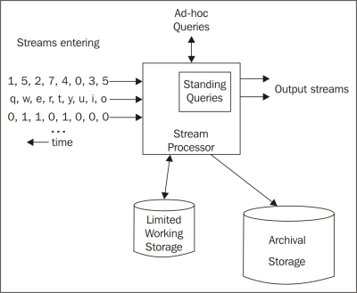
The STREAM algorithm is a classical algorithm used to cluster stream data. In the next section, the details are present and explained by R code.
The summarized pseudocode of the STREAM algorithm are as follows:

In the preceding algorithm, LOCALSEARCH is a revised k-median algorithm.


Please take a look at the R codes file ch_08_stream.R from the bundle of R codes for previously mentioned algorithms. The codes can be tested with the following command:
> source("ch_08_stream.R")
Day by day, the growing e-commerce market is driving the growth of the usage of credit card, which, in turn, is bringing in a large number of transaction streams. Fraudulent usage of credit cards happens every day; we want the algorithm to detect this kind of transaction in a very short time compared to the big volume of transactions. Besides this, the requirement to find out the valuable customers by an analysis of the transaction streams is becoming more and more important. However, it is harder to get valid information in a very short time in response to the advertisement needs, such as recommend the necessary finance services or goods to these customers.
The credit card transaction flow is also the process to generate stream data, and the related stream-mining algorithm can be applied with high accuracy.
One application for the credit card transaction flow mining is the behavior analysis of the consumers. With each transaction record that is stored, various costs or purchases of a certain person can be tracked. With the mining of such transaction records, we can provide an analysis to the credit card holder to help them keep financial balance or other financial target. We can also provide this analysis to the card issuer that published the credit card to create a new business, such as funding or loaning, or to the retailers (the merchants) such as Walmart to help in the arrangement of appropriate goods.
Another application for the credit card transaction flow mining is fraud detection. It is the most obvious one among tons of applications. Using this solution, the card issuer or the bank can reduce the rate of successful fraud.
The dataset of the credit card transaction includes the owner of cards, place of consumption, date, cost, and so on.
Auto Regressive Integrated Moving Average (ARIMA) is a classic algorithm to analyze time–series data. As the initial step, an ARIMA model will be chosen to model the time-series data. Assuming that  is a time-series variable such as a price, the formula is defined as follows, and it includes the main features of the variable:


Predicting future prices is one subproblem of predicting the future; this is just a sign of the difficulty of this issue. Another similar issue under this domain is estimating the future market demands.
The stock market is a good example of predicting the future price; here, the prices changes along with time. Predicting future prices helps estimate the equity returns in the future and also helps in deciding the timing for financial investors, such as when to buy/sell.
The price graph shows an oscillation. Many factors can affect this value, even the psycology of humans.
The key problem in this prediction is the huge data volume. As a direct result, the algorithms to be used for this topic need to be efficient. The other key problem is that the price might change dramatically in a short time. Also, the complexity of the market is definitely a big problem.
The data instances for the future price prediction include quantitative attributes such as technical factors, and they also include macroeconomics, microeconomics, political events, and investor expectations. Moreover, they include the domain expert's knowledge.
All the solutions based on the aggregate disperse information from the preselected factors.
Price is obviously affected by time, and is a time-series variable too. To forecast the future value, the time-series-analysis algorithm will apply. ARIMA can be used to forecast the prices of the next day.
One classical solution is to determine the trends of the market at a very early stage. Another solution is fuzzy solutions, which is also a good choice because of the huge volume of dataset and wide range of factors affecting the prices.
The ARIMA algorithm
Predicting future prices is one subproblem of predicting the future; this is just a sign of the difficulty of this issue. Another similar issue under this domain is estimating the future market demands.
The stock market is a good example of predicting the future price; here, the prices changes along with time. Predicting future prices helps estimate the equity returns in the future and also helps in deciding the timing for financial investors, such as when to buy/sell.
The price graph shows an oscillation. Many factors can affect this value, even the psycology of humans.
The key problem in this prediction is the huge data volume. As a direct result, the algorithms to be used for this topic need to be efficient. The other key problem is that the price might change dramatically in a short time. Also, the complexity of the market is definitely a big problem.
The data instances for the future price prediction include quantitative attributes such as technical factors, and they also include macroeconomics, microeconomics, political events, and investor expectations. Moreover, they include the domain expert's knowledge.
All the solutions based on the aggregate disperse information from the preselected factors.
Price is obviously affected by time, and is a time-series variable too. To forecast the future value, the time-series-analysis algorithm will apply. ARIMA can be used to forecast the prices of the next day.
One classical solution is to determine the trends of the market at a very early stage. Another solution is fuzzy solutions, which is also a good choice because of the huge volume of dataset and wide range of factors affecting the prices.
Predicting future prices
Predicting future prices is one subproblem of predicting the future; this is just a sign of the difficulty of this issue. Another similar issue under this domain is estimating the future market demands.
The stock market is a good example of predicting the future price; here, the prices changes along with time. Predicting future prices helps estimate the equity returns in the future and also helps in deciding the timing for financial investors, such as when to buy/sell.
The price graph shows an oscillation. Many factors can affect this value, even the psycology of humans.
The key problem in this prediction is the huge data volume. As a direct result, the algorithms to be used for this topic need to be efficient. The other key problem is that the price might change dramatically in a short time. Also, the complexity of the market is definitely a big problem.
The data instances for the future price prediction include quantitative attributes such as technical factors, and they also include macroeconomics, microeconomics, political events, and investor expectations. Moreover, they include the domain expert's knowledge.
All the solutions based on the aggregate disperse information from the preselected factors.
Price is obviously affected by time, and is a time-series variable too. To forecast the future value, the time-series-analysis algorithm will apply. ARIMA can be used to forecast the prices of the next day.
One classical solution is to determine the trends of the market at a very early stage. Another solution is fuzzy solutions, which is also a good choice because of the huge volume of dataset and wide range of factors affecting the prices.
Time-series clustering has been proven to provide effective information for further research. In contrast to the classic clustering, the time-series dataset comprises data changed with time.

This algorithm is denoted as "clustering seasonality patterns in the presence of errors"; the summarized algorithm is listed in the following figure. The major characteristic of this algorithm is to introduce a specific distance function and a dissimilarity function.

Please take a look at the R codes file ch_08_herror.R from the bundle of R codes for previously mentioned algorithms. The codes can be tested with the following command:
> source("ch_08_herror.R")
Stock market is a complex dynamic system, and many factors can affect the market. For example, breaking financial news is also a key factor for this topic.
The characteristics of stock market data are large volume (near infinite), real time, high dimensions, and high complexity. The various data streams from stock markets go along with many events and correlations.
Stock market sentiment analysis is one topic related to this domain. The stock market is too complex with many factors that can affect the market. People's opinion or sentiment is one of the major factors.
The real-time information needs from the stock market require the fast, efficient online-mining algorithms. The time-series data accounts for various data including the stock market data that updates along with time.
To predict the stock market, the past data is really important. Using the past return on certain stock, the future price of that stock can be predicted based on the price-data stream.
The hError algorithm
This algorithm is denoted as "clustering seasonality patterns in the presence of errors"; the summarized algorithm is listed in the following figure. The major characteristic of this algorithm is to introduce a specific distance function and a dissimilarity function.
Please take a look at the R codes file ch_08_herror.R from the bundle of R codes for previously mentioned algorithms. The codes can be tested with the following command:
> source("ch_08_herror.R")
Stock market is a complex dynamic system, and many factors can affect the market. For example, breaking financial news is also a key factor for this topic.
The characteristics of stock market data are large volume (near infinite), real time, high dimensions, and high complexity. The various data streams from stock markets go along with many events and correlations.
Stock market sentiment analysis is one topic related to this domain. The stock market is too complex with many factors that can affect the market. People's opinion or sentiment is one of the major factors.
The real-time information needs from the stock market require the fast, efficient online-mining algorithms. The time-series data accounts for various data including the stock market data that updates along with time.
To predict the stock market, the past data is really important. Using the past return on certain stock, the future price of that stock can be predicted based on the price-data stream.
Time-series classification with the 1NN classifier
The summarized pseudocode for the 1NN classifier algorithm is as follows:

Please take a look at the R codes file ch_08_herror.R from the bundle of R codes for previously mentioned algorithms. The codes can be tested with the following command:
> source("ch_08_herror.R")
Stock market is a complex dynamic system, and many factors can affect the market. For example, breaking financial news is also a key factor for this topic.
The characteristics of stock market data are large volume (near infinite), real time, high dimensions, and high complexity. The various data streams from stock markets go along with many events and correlations.
Stock market sentiment analysis is one topic related to this domain. The stock market is too complex with many factors that can affect the market. People's opinion or sentiment is one of the major factors.
The real-time information needs from the stock market require the fast, efficient online-mining algorithms. The time-series data accounts for various data including the stock market data that updates along with time.
To predict the stock market, the past data is really important. Using the past return on certain stock, the future price of that stock can be predicted based on the price-data stream.
The R implementation
Please take a look at the R codes file ch_08_herror.R from the bundle of R codes for previously mentioned algorithms. The codes can be tested with the following command:
> source("ch_08_herror.R")
Stock market is a complex dynamic system, and many factors can affect the market. For example, breaking financial news is also a key factor for this topic.
The characteristics of stock market data are large volume (near infinite), real time, high dimensions, and high complexity. The various data streams from stock markets go along with many events and correlations.
Stock market sentiment analysis is one topic related to this domain. The stock market is too complex with many factors that can affect the market. People's opinion or sentiment is one of the major factors.
The real-time information needs from the stock market require the fast, efficient online-mining algorithms. The time-series data accounts for various data including the stock market data that updates along with time.
To predict the stock market, the past data is really important. Using the past return on certain stock, the future price of that stock can be predicted based on the price-data stream.
Stock market data
Stock market is a complex dynamic system, and many factors can affect the market. For example, breaking financial news is also a key factor for this topic.
The characteristics of stock market data are large volume (near infinite), real time, high dimensions, and high complexity. The various data streams from stock markets go along with many events and correlations.
Stock market sentiment analysis is one topic related to this domain. The stock market is too complex with many factors that can affect the market. People's opinion or sentiment is one of the major factors.
The real-time information needs from the stock market require the fast, efficient online-mining algorithms. The time-series data accounts for various data including the stock market data that updates along with time.
To predict the stock market, the past data is really important. Using the past return on certain stock, the future price of that stock can be predicted based on the price-data stream.
Web click streams data is large and continuously emerging, with hidden trends buried and to be discovered for various usages, such as recommendations. TECNO-STREAMS (Tracking Evolving Clusters in NOisy Streams) is a one-pass algorithm.
The whole algorithm is modeled on the following equations: the robust weight or activation function (1), influence zone (2), pure simulation (3), optimal scale update (4), incremental update of pure simulation and optimal update (5) and (6), the simulation and scale values (7), and finally, the D-W-B-cell update equations (8).


The similarity measures applied in the learning phase are defined here:


The similarity measures applied in the validation phase are defined here:


The summarized pseudocode for the TECNO-STREAMS algorithm is as follows:

Please take a look at the R codes file ch_08_tecno_stream.R from the bundle of R codes for previous algorithm. The codes can be tested with the following command:
> source("ch_08_tecno_stream.R")
The web click streams denote the user's behavior when visiting the site, especially for e-commerce sites and CRM (Customer Relation Management). The analysis of web click streams will improve the user experience of the customer and optimize the structure of the site to meet the customers' expectation and, finally, increase the income of the site.
In other aspects, web click streams mining can be used to detect DoS attacks, track the attackers, and prevent these on the Web in advance.
The dataset for web click stream is obviously the click records that get generated when the user visits various sites. The major characteristics of this dataset are that it is huge, and the size goes on increasing.
The TECNO-STREAMS algorithm
The whole algorithm is modeled on the following equations: the robust weight or activation function (1), influence zone (2), pure simulation (3), optimal scale update (4), incremental update of pure simulation and optimal update (5) and (6), the simulation and scale values (7), and finally, the D-W-B-cell update equations (8).
The similarity measures applied in the learning phase are defined here:
The similarity measures applied in the validation phase are defined here:
The summarized pseudocode for the TECNO-STREAMS algorithm is as follows:
Please take a look at the R codes file ch_08_tecno_stream.R from the bundle of R codes for previous algorithm. The codes can be tested with the following command:
> source("ch_08_tecno_stream.R")
The web click streams denote the user's behavior when visiting the site, especially for e-commerce sites and CRM (Customer Relation Management). The analysis of web click streams will improve the user experience of the customer and optimize the structure of the site to meet the customers' expectation and, finally, increase the income of the site.
In other aspects, web click streams mining can be used to detect DoS attacks, track the attackers, and prevent these on the Web in advance.
The dataset for web click stream is obviously the click records that get generated when the user visits various sites. The major characteristics of this dataset are that it is huge, and the size goes on increasing.
The R implementation
Please take a look at the R codes file ch_08_tecno_stream.R from the bundle of R codes for previous algorithm. The codes can be tested with the following command:
> source("ch_08_tecno_stream.R")
The web click streams denote the user's behavior when visiting the site, especially for e-commerce sites and CRM (Customer Relation Management). The analysis of web click streams will improve the user experience of the customer and optimize the structure of the site to meet the customers' expectation and, finally, increase the income of the site.
In other aspects, web click streams mining can be used to detect DoS attacks, track the attackers, and prevent these on the Web in advance.
The dataset for web click stream is obviously the click records that get generated when the user visits various sites. The major characteristics of this dataset are that it is huge, and the size goes on increasing.
Web click streams
The web click streams denote the user's behavior when visiting the site, especially for e-commerce sites and CRM (Customer Relation Management). The analysis of web click streams will improve the user experience of the customer and optimize the structure of the site to meet the customers' expectation and, finally, increase the income of the site.
In other aspects, web click streams mining can be used to detect DoS attacks, track the attackers, and prevent these on the Web in advance.
The dataset for web click stream is obviously the click records that get generated when the user visits various sites. The major characteristics of this dataset are that it is huge, and the size goes on increasing.
Mining sequence patterns can be thought of as association discovery over the temporal data or sequence dataset. Similarly, the classic pattern-mining algorithm should be extended or modified as per the sequence dataset's scenario.

Here are some questions for you to know whether you have understood the concepts:
- What is a stream?
- What is a time series?
- What is a sequence?
In this chapter, you will learn the algorithms written in R for graph mining and network analysis.
In this chapter, we will cover the following topics:
- Graph mining
- Mining frequent subgraph patterns
- Social network mining
- Social influence mining
Grouping, messaging, dating, and many other means are the major forms of social communication or the classic social behavior in the social network. All these concepts are modeled with graphs; that is, nodes, edges, and other attributes. Graph mining is developed to mine this information, which is similar to other types of information, such as biological information, and so on.
Graph G contains nodes V and edges E and is represented with an equation, G = (V, E). As per graph mining, there are some concepts that need to be clarified. There are two types of graphs: directed graphs, which have ordered pairs of vertices in the edge set, E, and undirected graphs.
Although the data instances under research are very different from the other data types that we saw earlier in this book, graph-mining algorithms still include frequent pattern (subgraph) mining, classification, and clustering.
In the next section, we will look at frequent subgraph patterns mining algorithm, links mining, and clustering.
The subgraph pattern or graph pattern is an important application of data mining; this is used for bioinformatics, social network analysis, and so on. Frequent subgraph patterns are patterns that occur frequently in a set of graphs or in a large graph.

The gPLS algorithm

The GraphSig algorithm

Rightmost path extensions and their supports

The subgraph isomorphism enumeration algorithm

The canonical checking algorithm

Social network is based on human interactions, from the most classical definition. The data instances collected in the social network have graph-like and temporal characteristics. There are two major strategies for data mining tasks for social networks: one is linkage-based or structure-based, and the other is content-based. The data instances collected in the social network also have two kinds of data instances: static and dynamic or times-series data, such as the tweets on Twitter. Due to the characteristics of the data instance of graphs, there are vast versatile algorithms developed to solve the challenges.


Community detection and the shingling algorithm


Here are some practice questions for you to check whether you have understood the concepts:
- What is a graph?
- What graph opportunities are used?
- What is the PageRank algorithm, and what is its application in web search?
In this chapter, we looked at:
- Graph mining. We also saw that the characteristics of graph data can be divided into frequent pattern mining, classification, and clustering
- Mining frequent subgraph patterns is done to find the frequent patterns in a set of graphs or a single massive graph
- Social network analysis includes a wide range of web applications with broad definitions, such as Facebook, LinkedIn, Google+, StackOverflow, and so on
In the next chapter, we will focus on the major topics related to web mining and algorithms and look at some examples based on them.
In this chapter, you will learn the algorithm written in R for text mining and web data mining.
For text mining, the semistructured and nonstructured documents are the main dataset. There are a few of major categories of text mining, such as clustering, document retrieval and representation, and anomaly detection. The application of text mining includes, but is not limited to, topic tracking, and text summarization and categorization.
Web content, structure, and usage mining is one application of web mining. Web mining is also used for user behavior modeling, personalized views and content annotation, and so on. In another aspect, web mining integrates the result information from the traditional data-mining technologies and the information from WWW.
In this chapter, we will cover the following topics:
- Text mining and the TM package
- Text summarization
- The question answering system
- Genre categorization of web pages
- Categorization of newspaper articles and newswires into topics
- Web usage mining with web logs
Along with the appearance of text mining, due to the characteristics of text or documents, the traditional data-mining algorithms need some minor adjustments or extensions. The classical text-mining process is as follows:

The popular text-clustering algorithms include the distance-based clustering algorithm, the hierarchical clustering algorithm, the partition-based clustering algorithm, and so on.
The popular text-classification algorithms include decision trees, pattern-based classification, SVM classification, Bayesian classification, and so on.
As a popular preprocessing step, here are the details of the word-extraction algorithm.
The target of text summarization is to generate a concise and coherent conclusion or summary of the major information of the input. Three major steps are performed in most of the summarization systems. They are as follows:
- Build a temporary structure that contains the main portion of the key point of the input text.
- Next, the sentences from the input are scored with the output of the first step.
- Lastly, a final summary that represents the input documents is set up by several sentences.
One popular strategy is to remove the unimportant information, clauses, or sentences and, at the same time, build classifiers to make sure that the key information is not thrown away, which is, in another viewpoint, the relative importance of topics functioned here during the summarization process. The final result is represented in a coherent way.
The summarization is a dynamic nonstop process. First, we need to build summaries on the set of old documents' dataset, which means multidocuments' summarization. The second step is to summarize the new documents when we get the result of the first step.
Due to the difficulty in building a new sentence for the summaries, one solution is extractive summarization, that is, to extract the most relevant sentences from the document dataset or documents. With the growth of the size of the documents set, the time evolution of the topics is also an important issue for which statistical topic modeling such as time-series-based algorithms are proposed.
There are two popular solutions for intermediate representation: topic representation and indicator representation. Sentence scoring, the score of each sentence, is determined by a couple of important factors such as the combination of characters. Summary sentence selection is determined by the most important N sentences.
There are many good characteristics that describe the final summary: it is indicative or informative, extract or abstract, generic or query-oriented, consists of background or just the news, is monolingual or cross lingual, and consists of a single document or multiple documents.
The benefit of text summarization is to improve the efficiency of document processing during which the summarization of a certain document can help the reader decide whether to analyze the document for specific purposes. One example is to summarize the multilingual, large (nearing unlimited), dynamic dataset of documents from various sources, including the Web. Examples include summarization of medical articles, e-mail, the Web, speech, and so on.
Topic representation such as topic signature plays an important role in the document-summarization system. Various topic representations are provided, such as topic signature, enhanced topic signature, thematic signature, and so on.
The topic signature is defined as a set of related terms; topic is the target concept, and signature is a list of terms that is related to the topic with a specific weight. Each term can be the stemmed content words, bigram or trigram:

The topic term selection process is as follows. The input document sets are divided into two sets: relevant and nonrelevant texts for the topic. Two hypotheses are defined:


The first hypothesis denotes that the relevance of a document is independent of the term, whereas the second hypothesis indicates a strong relevance with the presence of those terms, given that  and the 2 x 2 contingency table:
|
R |

| |
|---|---|---|

|

|

|
|
|

|

|
represents the frequency of the term, , occurring in R, and , is the frequency of the term occurring in . is the frequency of the term,  , occurring in R, and is the frequency of the term, , occurring in .
The likelihood of both hypotheses is calculated as follows; here, b denotes the binomial distribution:


The algorithm to create the topic signature for a given topic is illustrated as follows:

Here is the Graph-Based Sub-topic Partition Algorithm (GSPSummary) algorithm for multidocument summarization:

The GSPRankMethod is defined as follows:

Maximal Marginal Relevance (MMR), which is comparatively suited for query-based and multidocument summarization, selects the most important sentence in each iteration of sentence selection. Each selected sentence has minimal relevance to the selected sentence set.

The summarized algorithm of MMR is as follows:

Topic representation
Topic representation such as topic signature plays an important role in the document-summarization system. Various topic representations are provided, such as topic signature, enhanced topic signature, thematic signature, and so on.
The topic signature is defined as a set of related terms; topic is the target concept, and signature is a list of terms that is related to the topic with a specific weight. Each term can be the stemmed content words, bigram or trigram:
The topic term selection process is as follows. The input document sets are divided into two sets: relevant and nonrelevant texts for the topic. Two hypotheses are defined:
The first hypothesis denotes that the relevance of a document is independent of the term, whereas the second hypothesis indicates a strong relevance with the presence of those terms, given that and the 2 x 2 contingency table:
|
R |
| |
|---|---|---|
|
|
|
|
|
|
|
|
represents the frequency of the term, , occurring in R, and , is the frequency of the term occurring in . is the frequency of the term, , occurring in R, and is the frequency of the term, , occurring in .
The likelihood of both hypotheses is calculated as follows; here, b denotes the binomial distribution:
The algorithm to create the topic signature for a given topic is illustrated as follows:
Here is the Graph-Based Sub-topic Partition Algorithm (GSPSummary) algorithm for multidocument summarization:
The GSPRankMethod is defined as follows:
Maximal Marginal Relevance (MMR), which is comparatively suited for query-based and multidocument summarization, selects the most important sentence in each iteration of sentence selection. Each selected sentence has minimal relevance to the selected sentence set.
The summarized algorithm of MMR is as follows:
The multidocument summarization algorithm
Here is the Graph-Based Sub-topic Partition Algorithm (GSPSummary) algorithm for multidocument summarization:
The GSPRankMethod is defined as follows:
Maximal Marginal Relevance (MMR), which is comparatively suited for query-based and multidocument summarization, selects the most important sentence in each iteration of sentence selection. Each selected sentence has minimal relevance to the selected sentence set.
The summarized algorithm of MMR is as follows:
The Maximal Marginal Relevance algorithm
Maximal Marginal Relevance (MMR), which is comparatively suited for query-based and multidocument summarization, selects the most important sentence in each iteration of sentence selection. Each selected sentence has minimal relevance to the selected sentence set.
The summarized algorithm of MMR is as follows:
The question answering (QA) system is a one hot topic related to IR, IE, NLP, data mining, and so on. A QA system mines a large set of texts to find a short phrase or sentence that answers a user's question with a certain precision. If the source is the Web or, even further, the whole information world, the challenge of the QA system increases dramatically.
There are basically three kinds of QA systems: slot filling, for which the format of the query and answer are similar; limited domain, for which the domains are limited with dictionaries and ontologies; and open domain, for which there is no limitation of domains.
One of the conceptual architectures among various solutions is illustrated in the following image. The input of the QA system is natural language questions; the output of the system, that is, the answer to the input question, is provided in natural language too. The system is composed of three major parts: the user interface, the processing part for questions, and the generation part for answers.
Assuming the question to be a coherent sentence, the questions from the user interface are processed, and the final right query is generated after a question-term identification, such as word segmentation and key word extraction and expansion. The ontology base here serves to support query expansion.
The answer is selected or generated from the FAQ base by the query that is provided in the earlier steps.

One popular question answering system is Yahoo! Answers, where a huge number of questions are asked and answered every day.
Genre categorization can be used for large article corpora and web pages. A genre can be defined in terms of purpose and physical form. It denotes any widely accepted categories of texts defined by common communicative purpose or other functional traits, and the categories are extensible. The web genre can also be defined based on the facets, complexity of the language, subjectivity, and number of graphics. Genre categorization has many applications such as improving search efficiency and satisfying the users' information need.
For the WWW or web pages, the genre can be defined as the usability of the miner and feasibility with respect to the efficiency.
There are some major challenges for this web page genre categorization. One is the instability of the Web itself. The second is the complex and unpredictable properties of web pages. The third is how to judge the genre for a specific web page. There are more challenges, but they are not listed here, or they will appear in future applications. For certain web pages, they might have multiple genres or no genre for existing recognized genres libraries.
Due to the fast pace of the evolution of the Web, new genres are continuously introduced to the current genre classes and the current genre classes are continuously updated and upgraded.
Possible solutions include, but are not limited to, Naïve Bayes, k-Nearest Neighbor, SVM, and tree nodes as classification methods.
Articles and newswires denote the huge periodical source of events of knowledge at different periods of time. The classification of text is the preprocessing step to store all these documents into a specific corpus. The categorization of text is the base of text processing.
We will now introduce an N-gram-based text-classification algorithm. From a longer string, an N-character slice is called N-gram. The key point of this algorithm is the calculation of the profiles of the N-gram frequencies.
Before the introduction of the algorithm, here are the necessary illustrations of a couple of concepts adopted in the algorithm:


Web usage mining denotes the discovery and analytics of patterns in web logs (such as system access logs) and transactions. The output is the relation of user interaction and resources on the Web. The user behavior can be identified based on this output. The web logs record the track of the web user's interaction with web servers, web proxy servers, and browsers.
The popular web usage mining process is illustrated in the images, and it includes three major steps: data collection and preprocessing, pattern discovery, and pattern analysis.
The preprocessing contains data cleaning, session identification, and data conversion. The pattern discovery includes path analysis, association rules, sequential patterns, and cluster and classification rules.


Here are some questions for you to know whether you have understood the concepts:
- What are the characteristics of text mining?
- What is the difference between text mining and data mining?
- What is the difference between web mining and data mining?
In this chapter, we looked at text mining, which is to find brand new or unknown information by extracting information from the documents dataset. We also looked at how text summarization presents the condensed result of the document set under research; in other words, takes a source, extracts contents, and presents the key contents in a condensed format that is sensitive to the final needs. Also, we looked at how genre classification discriminates between documents by form, style, and the targeted system or audience. We also covered the question answering system, topic detection, and web mining.
In this book, many useful data-mining algorithms are illustrated in the form of the R language, which has been there for years, even decades. The most popular algorithms are included with a detailed description. You can start working with the knowledge structure of the classical and living data-mining algorithms and solutions built with R.
Here is a list of algorithms related to association rules mining; it is only a small portion of the available algorithms, but it has proved to be effective:
|
Approach |
Dataset |
Sequential pattern mining |
Sequential rule mining |
Frequent itemset mining |
Association rule mining |
|---|---|---|---|---|---|
|
Apriori |
Transaction |
Yes | |||
|
AprioriTid |
Transaction |
Yes | |||
|
DHP (Direct Hashing and Pruning) |
Transaction |
Yes | |||
|
FDM (Fast Distributed Mining of association rules) |
Transaction |
Yes | |||
|
GSP (Generalized Sequential Patterns) |
Sequence |
Yes | |||
|
DIC |
Transaction |
Yes | |||
|
Pincer Search (the Pincer-search algorithm) |
Transaction |
Yes | |||
|
CARMA (Continuous Association Rule Mining Algorithm) |
Transaction |
Yes | |||
|
CHARM (Closed Association Rule Mining) |
Transaction |
Yes (closed) | |||
|
Depth-project |
Transaction |
Yes (maximal) | |||
|
Eclat |
Transaction |
Yes | |||
|
SPAD |
Sequence |
Yes | |||
|
SPAM |
Sequence |
Yes | |||
|
Diffset |
Transaction |
Yes | |||
|
FP-growth |
Transaction |
Yes |
FP-growth | ||
|
DSM-FI (Data Stream Mining for Frequent Itemsets) |
Transaction |
Yes | |||
|
PRICES |
Transaction |
Yes | |||
|
PrefixSpan |
Sequence |
Yes | |||
|
Sporadic Rules |
Transaction |
Yes | |||
|
IGB |
Transaction |
Yes | |||
|
GenMax |
Transaction |
Yes (maximal) | |||
|
FPMax (Frequent Maximal Item Set) |
Transaction |
Yes | |||
|
FHARM (Fuzzy Healthy Association Rule Mining) |
Transaction |
Yes | |||
|
H-Mine |
Transaction |
Yes | |||
|
FHSAR |
Transaction |
Yes | |||
|
Reverse Apriori |
Transaction |
Yes (maximal) | |||
|
DTFIM |
Transaction |
Yes | |||
|
GIT tree |
Transaction |
Yes | |||
|
Scaling Apriori |
Transaction |
Yes | |||
|
CMRules |
Sequence |
Yes | |||
|
Minimum effort |
Transaction |
Yes (maximal) | |||
|
TopSeqRules |
Sequence |
Yes | |||
|
FPG ARM |
Transaction |
Yes | |||
|
TNR |
Transaction |
Yes | |||
|
ClaSP |
Sequence |
Yes (closed) |