


In this chapter, we will cover the following recipes:
Installing packages and getting help in R
Data types in R
Special values in R
Matrices in R
Editing a matrix in R
Data frames in R
Editing a data frame in R
Importing data in R
Exporting data in R
Writing a function in R
Writing if else statements in R
Basic loops in R
Nested loops in R
The apply, lapply, sapply, and tapply functions
Using par to beautify a plot in R
Saving plots
If you are a new user and have never launched R, you must definitely start the learning process by understanding the use of install.packages(), library(), and getting help in R. R comes loaded with some basic packages, but the R community is rapidly growing and active R users are constantly developing new packages for R.
As you read through this cookbook, you will observe that we have used a lot of packages to create different visualizations. So the question now is, how do we know what packages are available in R? In order to keep myself up-to-date with all the changes that are happening in the R community, I diligently follow these blogs:
Rblogger
Rstudio blog
There are many blogs, websites, and posts that I will refer to as we go through the book. We can view a list of all the packages available in R by going to http://cran.r-project.org/, and also http://www.inside-r.org/packages provides a list as well as a short description of all the packages.
We can start by powering up our R studio, which is an Integrated Development Environment (IDE) for R. If you have not downloaded Rstudio, then I would highly recommend going to http://www.rstudio.com/ and downloading it.
To install a package in R, we will use the install.packages() function. Once we install a package, we will have to load the package in our active R session; if not, we will get an error. The library() function allows us to load the package in R.
The install.packages() function comes with some additional arguments but, for the purpose of this book, we will only use the first argument, that is, the name of the package. We can also load multiple packages by using install.packages(c("plotrix", "RColorBrewer")). The name of the package is the only argument we will use in the library() function. Note that you can only load one package at a time with the library() function unlike the install.packages() function.
It is hard to remember all the functions and their arguments in R, unless we use them all the time, and we are bound to get errors and warning messages. The best way to learn R is to use the active R community and the help manual available in R.
To understand any function in R or to learn about the various arguments, we can type ?<name of the function>. For example, I can learn about all the arguments related to the plot() function by simply typing ?plot or ?plot() in the R console window. You will now view the help page on the right side of the screen. We can also learn more about the behavior of the function using some of the examples at the bottom of the help page.
If we are still unable to understand the function or its use and implementation, we could go to Google and type the question or use the Stack Overflow website. I am always able to resolve my errors by searching on the Internet. Remember, every problem has a solution, and the possibilities with R are endless.
Flowing Data (http://flowingdata.com/): This is a good resource to learn visualization tools and R. The tutorials are based on an annual subscription.
Stack Overflow (http://stackoverflow.com/): This is a great place to get help regarding R functions.
Inside-R (http://www.inside-r.org/): This lists all the packages along with a small description.
Rblogger (http://www.r-bloggers.com/): This is a great webpage to learn about new R packages, books, tutorials, data scientists, and other data-related jobs.
R forge (https://r-forge.r-project.org/).
R journal (http://journal.r-project.org/archive/2014-1/).
Everything in R is in the form of objects. Objects can be manipulated in R. Some of the common objects in R are numeric vectors, character vectors, complex vectors, logical vectors, and integer vectors.
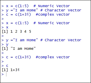
In order to generate a numeric vector in R, we can use the C() notation to specify it as follows:
x = c(1:5) # Numeric Vector
To generate a character vector, we can specify the same within quotes (" ") as follows:
y ="I am Home" # Character Vector
To generate a complex vector, we can use the i notation as follows:
c = c(1+3i) #complex vector
A list is a combination of a character and a numeric vector and can be specified using the list() notation:
z = list(c(1:5),"I am Home") # List
R comes with some special values. Some of the special values in R are NA, Inf, -Inf, and NaN.
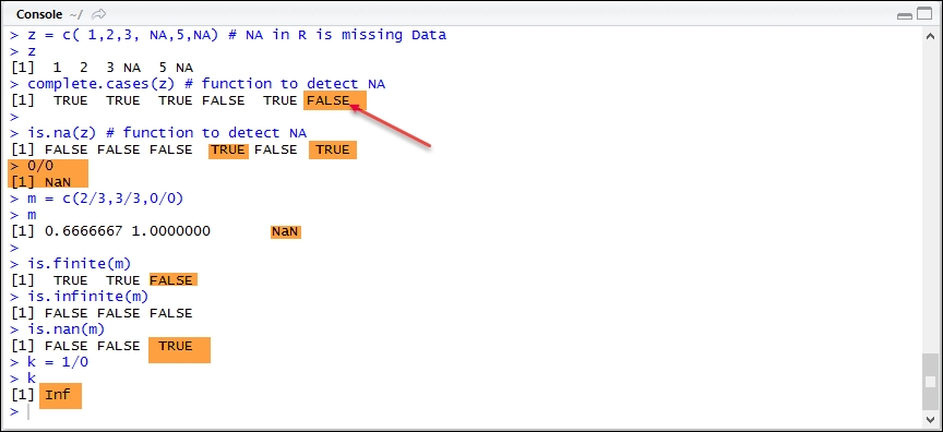
The missing values are represented in R by NA. When we download data, it may have missing data and this is represented in R by NA:
z = c( 1,2,3, NA,5,NA) # NA in R is missing Data
To detect missing values, we can use the install.packages() function or is.na(), as shown:
complete.cases(z) # function to detect NAis.na(z) # function to detect NA
To remove the NA values from our data, we can type the following in our active R session console window:
clean <- complete.cases(z)
z[clean] # used to remove NA from data
Please note the use of square brackets ([ ]) instead of parentheses.
In R, not a number is abbreviated as NaN. The following lines will generate NaN values:
##NaN
0/0
m <- c(2/3,3/3,0/0)
m
The is.finite, is.infinite, or is.nan functions will generate logical values (TRUE or FALSE).
is.finite(m)
is.infinite(m)
is.nan(m)
The following line will generate inf as a special value in R:
## infinite
k = 1/0
Tip
Downloading the example code
You can download the example code files for all Packt books you have purchased from your account at http://www.packtpub.com. If you purchased this book elsewhere, you can visit http://www.packtpub.com/support and register to have the files e-mailed directly to you.
complete.cases(z) is a logical vector indicating complete cases that have no missing value (NA). On the other hand, is.na(z) indicates which elements are missing. In both cases, the argument is our data, a vector, or a matrix.
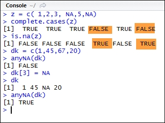
R also allows its users to check if any element in a matrix or a vector is NA by using the anyNA() function. We can coerce or assign NA to any element of a vector using the square brackets ([ ]). The [3] input instructs R to assign NA to the third element of the dk vector.
In this recipe, we will dive into R's capability with regard to matrices.
A vector in R is defined using the c() notation as follows:
vec = c(1:10)
A vector is a one-dimensional array. A matrix is a multidimensional array. We can define a matrix in R using the matrix() function. Alternatively, we can also coerce a set of values to be a matrix using the as.matrix() function:
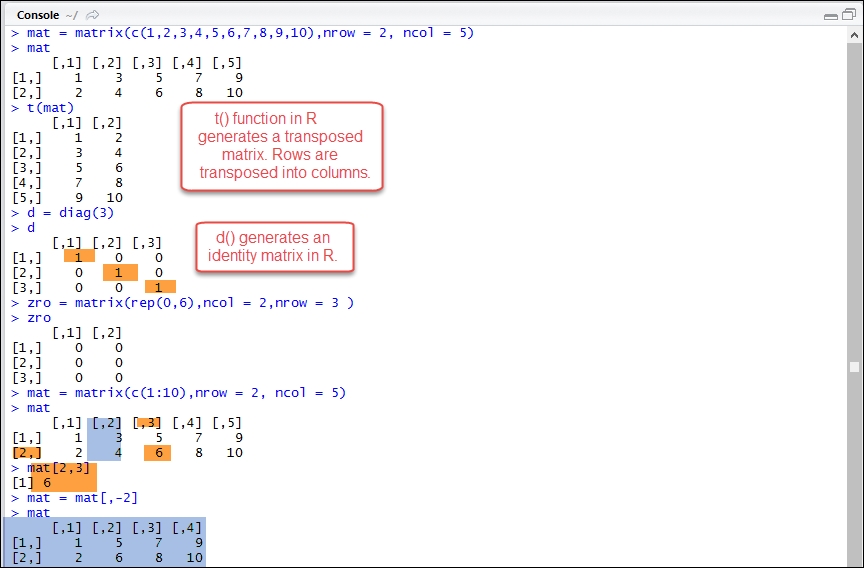
mat = matrix(c(1,2,3,4,5,6,7,8,9,10),nrow = 2, ncol = 5)
mat
To generate a transpose of a matrix, we can use the t() function:
t(mat) # transpose a matrix
In R, we can also generate an identity matrix using the diag() function:
d = diag(3) # generate an identity matrix
We can nest the rep () function within matrix() to generate a matrix with all zeroes as follows:
zro = matrix(rep(0,6),ncol = 2,nrow = 3 )# generate a matrix of Zeros
zro
We can define our data in the matrix () function by specifying our data as its first argument. The nrow and ncol arguments are used to specify the number of rows and column in a matrix. The matrix function in R comes with other useful arguments and can be studied by typing ?matrix in the R command window.
The rep() function nested in the matrix() function is used to repeat a particular value or character string a certain number of times.
The diag() function can be used to generate an identity matrix as well as extract the diagonal elements of a matrix. More uses of the diag() function can be explored by typing ?diag in the R console window.
The code file provides a lot more functions that can used along with matrices—for example, functions related to finding a determinant or inverse of a matrix and matrix multiplication.
R allows us to edit (add, delete, or replace) elements of a matrix using the square bracket notation, as depicted in the following lines of code:
mat = matrix(c(1:10),nrow = 2, ncol = 5)
mat
mat[2,3]
In order to extract any element of a matrix, we can specify the position of that element in R using square brackets. For example, mat[2,3] will extract the element under the second row and the third column. The first numeric value corresponds to the row and the second numeric value corresponds to a column [row, column].
Similarly, to replace an element, we can type the following lines in R:
mat[2,3] = 16
To select all the elements of the second row, we can use mat[2, ]. If we do not specify any numeric value for a column, R will automatically assume all columns.
One of the useful and widely used functions in R is the data.frame() function. Data frame, according to the R manual, is a matrix structure whose columns can be of differing types, such as numeric, logical, factor, or character.
A data frame in R is a collection of variables. A simple way to construct a data frame is using the data.frame() function in R:
data = data.frame(x = c(1:4), y = c("tom","jerry","luke","brian"))
data
Many times, we will encounter plotting functions that require data to be in a data frame. In order to coerce our data into a data frame, we can use the data.frame() function. In the following example, we create a matrix and convert it into a data frame:
mat = matrix(c(1:10), nrow = 2, ncol = 5)
data.frame(mat)
The data.frame() function comes with various arguments and can be explored by typing ?data.frame in the R console window. The code file under the title Data Frames – 2 provides additional functions that can help in understanding the underlying structure of our data. We can always get additional help by using the R documentation.
Once we have generated a data and converted it into a data frame, we can edit any row or column of a data frame.
We can add or extract any column of a data frame using the dollar ($) symbol, as depicted in the following code:
data = data.frame(x = c(1:4), y = c("tom","jerry","luke","brian"))
data$age = c(2,2,3,5)
data
In the preceding example, we have added a new column called age using the $ operator. Alternatively, we can also add columns and rows using the rbind() and cbind() functions in R as follows:
age = c(2,2,3,5)
data = cbind(data, age)
The cbind and rbind functions can also be used to add columns or rows to an existing matrix.
To remove a column or a row from a matrix or data frame, we can simply use the negative sign before the column or row to be deleted, as follows:
data = data[,-2]
The data[,-2] line will delete the second column from our data.
To re-order the columns of a data frame, we can type the following lines in the R command window:
data = data.frame(x = c(1:4), y = c("tom","jerry","luke","brian"))
data = data[c(2,1)]# will reorder the columns
data
To view the column names of a data frame, we can use the names() function:
names(data)
To rename our column names, we can use the colnames() function:
colnames(data) = c("Number","Names")Data comes in various formats. Most of the data available online can be downloaded in the form of text documents (.txt extension) or as comma-separated values (.csv). We also encounter data in the tab-delimited format, XLS, HTML, JSON, XML, and so on. If you are interested in working with data, either in JSON or XML, refer to the recipe Constructing a bar plot using XML in R in Chapter 10, Creating Applications in R.
In order to import a CSV file in R, we can use the read.csv() function:
test = read.csv("raw.csv", sep = ",", header = TRUE)Alternatively, read.table() function allows us to import data with different separators and formats. Following are some of the methods used to import data in R:
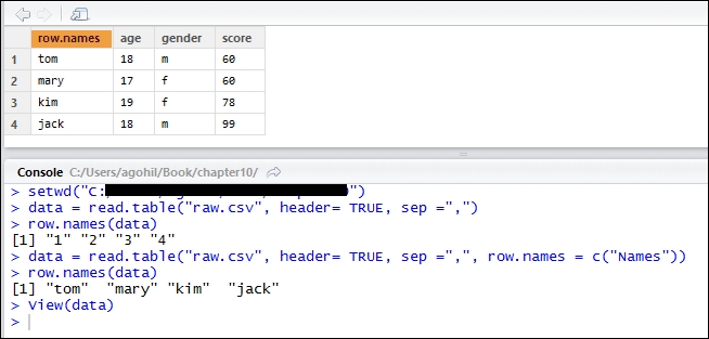
The first argument in the read.csv() function is the filename, followed by the separator used in the file. The header = TRUE argument is used to instruct R that the file contains headers. Please note that R will search for this file in its current directory. We have to specify the directory containing the file using the setwd() function. Alternatively, we can navigate and set our working directory by navigating to Sessions | Set working directory | Choose directory.
The first argument in the read.table() function is the filename that contains the data, the second argument states that the data contains the header, and the third argument is related to the separator. If our data consists of a semi colon (;), a tab delimited, or the @ symbol as a separator, we can specify this under the sep ="" argument. Note that, to specify a separator as a tab delimited, users would have to substitute sep = "," with sep ="\t" in the read.table() function.
One of the other useful arguments is the row.names argument. If we omit row.names, R will use the column serial numbers as row.names. We can assign row.names for our data by specifying it as row.names = c("Name").
Once we have processed our data, we need to save it to an external device or send it to our colleagues. It is possible to export data in R in many different formats.
To export data from R, we can use the write.table() function. Please note that R will export the data to our current directory or the folder we have assigned using the setwd() function:
write.table(data, "mydata.csv", sep=",")
The first argument in the write.table() function is the data in R that we would like to export. The second argument is the name of the file. We can export data in the .xls or .txt format, simply by replacing the mydata.csv file extension with mydata.txt or mydata.xls in the write.table() function.
Most of the tasks in R are performed using functions. A function in R has the same utility as functions in Arithmetic.
In order to write a simple function in R, we must first open a new R script by navigating to File | New file.
We write a very simple function that accepts two values and adds them together. Copy and paste the code in the new blank R script:
add = function (x,y){
  x+y
}A function in R should be defined by function(). Once we define our function, we need to save it as a .r file. Note that the name of the file should be the same as the function; hence we save our function with name add.r.
In order to use the add() function in the R command window, we need to source the file by using the source() function as follows:
source('<your path>/add.R')Now, we can type add(2,15) in the R command window. You get 17 printed as an output.
The function itself takes two arguments in our recipe but, in reality, it can take many arguments. Anything defined inside curly braces gets executed when we call add(). In our case, we request the user to input two variables, and the output is a simple sum.
Functions can be helpful in performing repetitive tasks such as generating plots or perform complicated calculations. Felix Schönbrodt has implemented visually weighted watercolor plots in R using a function on his blog at http://www.nicebread.de/visually-weighted-watercolor-plots-new-variants-please-vote/.
We can generate similar plots simply by copying the function created by Felix in our R session and executing it. The plotting function created by Felix also provides users with different ways in which the R function's ability could be leveraged to perform repetitive tasks.
We often use if statements in MS Excel, but we can also write a small code to perform simple tasks in R.
The logic for if else statements is very simple and is as follows:
if(x>3){
  print("greater value")
}else {
  print("lesser value")
}
We can copy and paste the preceding statement in the R console or write a function that makes use of the if else logic.
The logic behind if else statements is very simple. The following lines clearly state the logic:
if(condition){
#perform some action
}else {
  #perform some other action
}
The preceding code will check whether x is greater than or less than 3, and simply print it. In order to get the value, we type the following in the R command window:
x = 2
We can nest loops, as well as if statements, to perform some more complicated tasks. In this recipe, we will first define a square matrix and then write a nested for loop to print only those values where I = J, namely, the values in the matrix placed in (1,1), (2,2), and so on.
We first define a matrix in R using the following matrix() function:
mat= matrix(1:25, 5,5)
Now, we use the following code to output only those elements where I = J:
for (i in 1:5){
  for (j in 1:5){
    if (i ==j){
      print(mat[i,j])
    }
   }
}
The if statement is nested inside two for loop statements. As we have a matrix, we have to use two for loops instead of just one. The output of the matrix would be values such as 1, 7, 13, and 19.
R has some very handy functions such as
apply, sapply, tapply, and mapply, that can be used to reduce the task of writing complicated statements. Also, using them makes our code look cleaner. The apply() function is similar to writing a loop statement.
The lapply() function is very similar to the apply() function but can be used on lists; this will return a list. The sapply() function is very similar to lapply() but returns a vector and not a list.
The apply() function can be used as follows:
mat= matrix(1:25, 5,5)
apply(mat,1,sd)
The lapply() function can be used in the following way:
j = list(x = 1:4, b = rnorm(100,1,2))
lapply(j,mean)
The tapply() function is useful when we have broken a vector into factors, groups, or categories:
tapply(mtcars$mpg,mtcars$gear,mean)
The first argument in the apply() function is the data. The second argument takes two values: 1 and 2; if we state 1, R will perform a row-wise computation; if we mention 2, R will perform a column-wise computation. The third argument is the function. We would like to calculate the standard deviation of each row in R; hence we use the sd function as the third argument. Note that we can define our own function and replace it with the sd function.
With regard to the lapply() function, we have defined J as a list and would like to calculate the mean. The first argument in the lapply() function is the data and the second argument is the function used to process the data.
The first argument in the tapply() function is the data; in our case it is mpg. The second argument is the factor or the grouping; in this case it would be gears. The last argument is the function used to process the data. We would like to calculate the mean of mpg for each unique gear (3, 4, and 5 gears) in the mtcars data.
One quick and easy way to edit a plot is by generating the plot in R and then using Inkspace or any other software to edit it. We can save some valuable time if we know some basic edits that can be applied on a plot by setting them in a par() function. All the available options to edit a plot can be studied in detail by typing ?par in the command window.
In the following code, I have highlighted some commonly used parameters:
x=c(1:10)
y=c(1:10)
par(bg = "#646989", las = 1, col.lab = "black", col.axis = "white",bty = "n",cex.axis = 0.9,cex.lab= 1.5)
plot(x,y, pch = 20, xlab = "fake x data", ylab = "fake y data")
Under the par() function, we have set the background color using the bg = argument. The las = argument changes the orientation of the labels. The col.lab and col.axis arguments are used to specify the color of the labels as well as the axis. The cex argument is used to specify the size of the labels and axis. The bty argument is used to specify the box style in R.
We can save a plot in various formats, such as .jpeg, .svg, .pdf, or .png. I prefer saving a plot as a .png file, as it is easier to edit a plot with Inkspace if saved in the PNG format.
To save a plot in the .png format, we can use the png() function as follows:
png("TEST.png", width = 300, height = 600)
plot(x,y, xlab = "x axis", ylab = "y axis", cex.lab = 3,col.lab = "red", main = "some data", cex.main=1.5, col.main = "red")
dev.off()We have used the png() function to save the plot as a PNG. To save a plot as a PDF, SVG, or JPEG, we can use the pdf(), svg(), or jpeg() functions, respectively.
The first argument in the png() function is the name of the file with the extension, followed by the width and height of the plot. We can now use the plot() function to generate a plot; any subsequent plots will also be saved with a .png extension, unless the dev.off() function is passed. The dev.off() function instructs R that we do not need to save the plots.


