Home Programming Quantum Computing with Silq Programming

Quantum Computing with Silq Programming

By Srinjoy Ganguly , Thomas Cambier
books-svg-icon Book
eBook $29.99 $20.98
Print $43.99
Subscription $15.99 $10 p/m for three months
$10 p/m for first 3 months. $15.99 p/m after that. Cancel Anytime!
What do you get with a Packt Subscription?
This book & 7000+ ebooks & video courses on 1000+ technologies
60+ curated reading lists for various learning paths
50+ new titles added every month on new and emerging tech
Early Access to eBooks as they are being written
Personalised content suggestions
Customised display settings for better reading experience
50+ new titles added every month on new and emerging tech
Playlists, Notes and Bookmarks to easily manage your learning
Mobile App with offline access
What do you get with a Packt Subscription?
This book & 6500+ ebooks & video courses on 1000+ technologies
60+ curated reading lists for various learning paths
50+ new titles added every month on new and emerging tech
Early Access to eBooks as they are being written
Personalised content suggestions
Customised display settings for better reading experience
50+ new titles added every month on new and emerging tech
Playlists, Notes and Bookmarks to easily manage your learning
Mobile App with offline access
What do you get with eBook + Subscription?
Download this book in EPUB and PDF formats, plus a monthly download credit
This book & 6500+ ebooks & video courses on 1000+ technologies
60+ curated reading lists for various learning paths
50+ new titles added every month on new and emerging tech
Early Access to eBooks as they are being written
Personalised content suggestions
Customised display settings for better reading experience
50+ new titles added every month on new and emerging tech
Playlists, Notes and Bookmarks to easily manage your learning
Mobile App with offline access
What do you get with a Packt Subscription?
This book & 6500+ ebooks & video courses on 1000+ technologies
60+ curated reading lists for various learning paths
50+ new titles added every month on new and emerging tech
Early Access to eBooks as they are being written
Personalised content suggestions
Customised display settings for better reading experience
50+ new titles added every month on new and emerging tech
Playlists, Notes and Bookmarks to easily manage your learning
Mobile App with offline access
What do you get with eBook?
Download this book in EPUB and PDF formats
Access this title in our online reader
DRM FREE - Read whenever, wherever and however you want
Online reader with customised display settings for better reading experience
What do you get with video?
Download this video in MP4 format
Access this title in our online reader
DRM FREE - Watch whenever, wherever and however you want
Online reader with customised display settings for better learning experience
What do you get with video?
Stream this video
Access this title in our online reader
DRM FREE - Watch whenever, wherever and however you want
Online reader with customised display settings for better learning experience
What do you get with Audiobook?
Download a zip folder consisting of audio files (in MP3 Format) along with supplementary PDF
What do you get with Exam Trainer?
Flashcards, Mock exams, Exam Tips, Practice Questions
Access these resources with our interactive certification platform
Mobile compatible-Practice whenever, wherever, however you want
BUY NOW $10 p/m for first 3 months. $15.99 p/m after that. Cancel Anytime!
eBook $29.99 $20.98
Print $43.99
Subscription $15.99 $10 p/m for three months
What do you get with a Packt Subscription?
This book & 7000+ ebooks & video courses on 1000+ technologies
60+ curated reading lists for various learning paths
50+ new titles added every month on new and emerging tech
Early Access to eBooks as they are being written
Personalised content suggestions
Customised display settings for better reading experience
50+ new titles added every month on new and emerging tech
Playlists, Notes and Bookmarks to easily manage your learning
Mobile App with offline access
What do you get with a Packt Subscription?
This book & 6500+ ebooks & video courses on 1000+ technologies
60+ curated reading lists for various learning paths
50+ new titles added every month on new and emerging tech
Early Access to eBooks as they are being written
Personalised content suggestions
Customised display settings for better reading experience
50+ new titles added every month on new and emerging tech
Playlists, Notes and Bookmarks to easily manage your learning
Mobile App with offline access
What do you get with eBook + Subscription?
Download this book in EPUB and PDF formats, plus a monthly download credit
This book & 6500+ ebooks & video courses on 1000+ technologies
60+ curated reading lists for various learning paths
50+ new titles added every month on new and emerging tech
Early Access to eBooks as they are being written
Personalised content suggestions
Customised display settings for better reading experience
50+ new titles added every month on new and emerging tech
Playlists, Notes and Bookmarks to easily manage your learning
Mobile App with offline access
What do you get with a Packt Subscription?
This book & 6500+ ebooks & video courses on 1000+ technologies
60+ curated reading lists for various learning paths
50+ new titles added every month on new and emerging tech
Early Access to eBooks as they are being written
Personalised content suggestions
Customised display settings for better reading experience
50+ new titles added every month on new and emerging tech
Playlists, Notes and Bookmarks to easily manage your learning
Mobile App with offline access
What do you get with eBook?
Download this book in EPUB and PDF formats
Access this title in our online reader
DRM FREE - Read whenever, wherever and however you want
Online reader with customised display settings for better reading experience
What do you get with video?
Download this video in MP4 format
Access this title in our online reader
DRM FREE - Watch whenever, wherever and however you want
Online reader with customised display settings for better learning experience
What do you get with video?
Stream this video
Access this title in our online reader
DRM FREE - Watch whenever, wherever and however you want
Online reader with customised display settings for better learning experience
What do you get with Audiobook?
Download a zip folder consisting of audio files (in MP3 Format) along with supplementary PDF
What do you get with Exam Trainer?
Flashcards, Mock exams, Exam Tips, Practice Questions
Access these resources with our interactive certification platform
Mobile compatible-Practice whenever, wherever, however you want
  1. Free Chapter
    Chapter 1: Essential Mathematics and Algorithmic Thinking
About this book
Quantum computing is a growing field, with many research projects focusing on programming quantum computers in the most efficient way possible. One of the biggest challenges faced with existing languages is that they work on low-level circuit model details and are not able to represent quantum programs accurately. Developed by researchers at ETH Zurich after analyzing languages including Q# and Qiskit, Silq is a high-level programming language that can be viewed as the C++ of quantum computers! Quantum Computing with Silq Programming helps you explore Silq and its intuitive and simple syntax to enable you to describe complex tasks with less code. This book will help you get to grips with the constructs of the Silq and show you how to write quantum programs with it. You’ll learn how to use Silq to program quantum algorithms to solve existing and complex tasks. Using quantum algorithms, you’ll also gain practical experience in useful applications such as quantum error correction, cryptography, and quantum machine learning. Finally, you’ll discover how to optimize the programming of quantum computers with the simple Silq. By the end of this Silq book, you’ll have mastered the features of Silq and be able to build efficient quantum applications independently.
Publication date:
April 2021
Publisher
Packt
Pages
310
ISBN
9781800569669


Chapter 1: Essential Mathematics and Algorithmic Thinking

Quantum computing utilizes the phenomena and properties of quantum mechanics to perform computational tasks. This is done using a quantum computer, which is made using the principles of quantum physics. Today, quantum computers are still in their early stages, but the field is rapidly evolving as more and more communities from different backgrounds get involved in the field. Quantum computers will soon be able to solve challenges that are too complex for classical computers.

This chapter is intended to develop your understanding of the mathematical concepts that are required for quantum computing. This will help you to understand the ideas behind the applications of mathematical concepts to quantum computation. We will cover the following topics:

  • Linear algebra
  • Coordinate systems, probability, and complex numbers
  • Computational thinking and computer algorithms
  • The time and space complexity of algorithms
 

Introducing linear algebra for quantum computing

The concepts and techniques of linear algebra are so important and central to the field of quantum computing because almost all of the operations that take place in quantum computing use the language of linear algebra to describe the details and processes that happen within a quantum computer.

Linear algebra deals with the study of vector spaces and matrices. It primarily covers linear mapping and transformations of vectors and matrices. The geometric representation of linear algebra, such as in 2D Cartesian systems, makes it a lot easier to visualize operations happening on vectors and matrices.

In this section, we will cover the essential topics of linear algebra that are relevant to the world of quantum computing. The mathematical terms will be related to their equivalent quantum computing terms so that you can get a full understanding of the technical terms in quantum language. Let's start with the basic building blocks of linear algebra – vectors and vector spaces.

Vectors and vector spaces

In this section, you will develop a fundamental understanding of vectors and vector spaces. You will also learn about the relationship between vectors and the quantum computing world and will come to appreciate the practical nature of the mathematics involved. In quantum computing and quantum mechanics, vector spaces constitute all the possible quantum states, and they obey the rules of addition and multiplication. Vectors and vector spaces also play an important role in fluid mechanics, wave propagation, and oscillators.

Vectors

In the world of classical computation, we represent classical bits as 0, which represents the voltage level being off, and 1, which represents it being on. However, in the world of quantum computing, we use the term qubit, or quantum bit, to represent bits. Quantum bits comprise a two-level quantum system that forms the basic units of information in quantum computation, and they derive their properties from quantum mechanics. You may wonder why I am discussing qubits in the vectors section; this is because qubits can be represented as vectors!

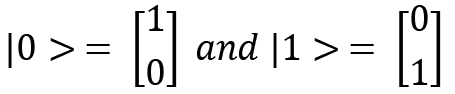
Vectors are just collections or lists of numbers, and in a more geometric sense, they represent direction along with magnitude. Mathematicians refer to these as vectors, whereas quantum physicists and computer scientists call them qubits. I will use the term qubits instead of vectors. The notation to represent qubits is known as the bra-ket notation or Dirac notation and uses angle brackets, <>, and vertical bars, |, to represent the qubits. The paper by Dirac titled A new notation for quantum mechanics explains the bra-ket notation in more detail and can be found in the Further reading section. The basic qubits used most frequently in quantum computing are column vectors (2D).

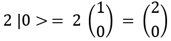
The 0 qubit can be written as and 1 can be written as ; these are called ket 0 and ket 1, respectively. Qubits are quantum states, and a general quantum state can be denoted by .

We can see a ket representation of qubits as follows:

The bra notation, which is the transpose of ket, is given as follows:

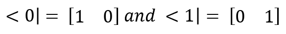
The important properties of the bra-ket notation is as follows:

  • Every ket qubit will have a bra qubit.
  • Constant multiple property – for a constant multiple c, , and .

Vector spaces

A vector space is a collection of vectors where two essential operations can take place, namely, vector addition and scalar multiplication. In quantum computing, you deal with complex vector spaces, , called Hilbert spaces, which means that vectors can consist of complex numbers, and all the rules of complex numbers can be applied in the calculations whenever we are carrying out operations and calculations with vectors and matrices. Hilbert spaces are usually denoted by the letter H. We will see this more in the next section.

Vector addition can be performed in the following way:

Here, the corresponding elements of the vectors are added together. This can be easily extended to dimensions as well, where corresponding elements are added. The quantum state formed previously is also known as a superposition of quantum states, which means that not only can quantum states be present at or , but they can also be present in the superposition of and . This is a very important property in quantum computation. Superposition states are linear combinations of other quantum states.

According to quantum mechanics, quantum states always need to be normalized because the probabilistic description of wave functions in quantum mechanics means that all the probabilities add to 1, so normalizing the state will give us , which is the proper definition of the state . The modulus squared of the coefficients of the quantum states gives us the probability of finding that particular state. As an example, is the respective probabilities of finding and in the preceding case.

Scalar multiplication in vector spaces happens as follows:

Here the scalar, which can be a real or complex number, is being multiplied by each of the elements present in the vector.

Whenever a vector can be written as a linear combination of other vectors, those vectors are known as linearly dependent vectors. Therefore, the linear independence of vectors implies that vectors cannot be written as a combination of other vectors. For example, the vectors and are linearly independent, but is linearly dependent because can be written as . The vectors and form the basis vectors and are the most common computational basis used in quantum computation. Similarly, in terms of Cartesian coordinates, the vectors (1, 0) and (0, 1) form the basis vectors for the Cartesian plane.

Vectors and vector spaces are very important concepts and will be used frequently throughout the book. We will now describe some operations that are important for vectors.

Inner products and norms

Inner products is a useful concept for the comparison of closeness between two vectors or quantum states, which is frequently carried out in quantum computing. In this section, you will become familiar with the calculation of inner products and the norms of quantum states. Inner products are useful for identifying the distinguishability of two different quantum states, and this property can be used for clustering. Norms are useful for describing the stretch or range of a particular quantum state in the vector space.

Inner products

The most important difference between an inner product and a dot product is the space and the mapping process. For the dot product, you will be familiar with the fact that the process takes two vectors from the Euclidean space and operates on them to provide us with a real number. In the case of inner products, the two vectors are taken from the space and the operations map it to a complex number. Inner products measure the closeness between two vectors. The notation <a|b> defines an inner product between two quantum states or two vectors.

For calculating, we have , where is the transpose of vector a. If , then the vectors are known as orthogonal vectors. Since the output of the inner product is complex, holds true.

Let's solve an example to see the calculation of inner products:

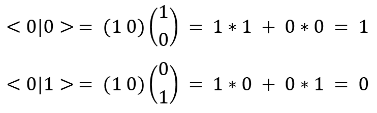
Similarly, you can verify that and Since , it shows that and are orthogonal, but , which shows that they are normalized. This means that and are orthonormal!

For the calculation of the inner product whenever the elements are complex, the Hermitian conjugate of the vector is necessary to compute. To calculate the Hermitian conjugate, we take the complex conjugate of the elements of the vector and write it in a row vector form. For the computation of inner products, we then multiply the Hermitian conjugate by the column vector. The Hermitian conjugate is denoted by .

Norms

The norm of a vector gives us the length of that vector. This is a real number and is denoted as follows:

The notion of the length of a vector is also known as the magnitude of the vector, which was mentioned at the beginning of the section on vectors. These operations are important for understanding various quantum algorithms in later chapters.

With inner products, norms, and vector spaces defined, let's now look at a few properties of Hilbert spaces, which are where all quantum computations happen.

Properties of Hilbert spaces

Let's look at some important properties of Hilbert spaces very briefly. You can try solving the proofs of these properties for yourself as a nice exercise:

  • A Hilbert space is a linear vector space satisfying the inner product condition –
  • Hilbert spaces satisfy conjugate symmetry:
  • Hilbert spaces satisfy positive definiteness:
  • Hilbert spaces are separable, so they contain a countable dense subset.
  • Hilbert spaces satisfy that they are linear with respect to the first vector: where are scalars.
  • Hilbert spaces satisfy that they are anti-linear with respect to the second vector:

We have discussed the various characteristics of and operations for vectors. Now we will dive into matrices and their operations while describing their relevance to quantum computing.

Matrices and their operations

Matrices are a significant part of quantum computing and their importance can't be emphasized enough. The fundamental concept behind matrices is that they connect theoretical quantum computing with practical quantum computing because they are easily implemented on computers for calculations. In this section, you will learn about matrices and their operations.

A matrix is an array of numbers that are arranged in a tabular format, that is, in the form of rows and columns. Primarily, matrices represent linear transformations in a vector space, making them essentially a process of linear mappings between vector spaces. For example, a rotation matrix is a rectangular array of elements arranged in order to rotate a vector in a 2D or 3D space. From this, you should begin to grasp the idea that whenever a matrix acts on an object, it will create some effect, and the effect is usually in the form of the transformation of functions or spaces. So, matrices can be called operators in the language of quantum computation, or in other words, operators can be represented using matrices.

The general form of a matrix is as follows:

Here represents the element at the row and the column. When , if the rows and the columns equal each other, then that matrix is known as a square matrix.

Since we are now familiar with the matrix notation, let's dive into some basic operations that are performed on matrices for simple calculations. Along the way, we will keep on seeing other forms of matrices that are important to the field of quantum computing.

Transpose of a matrix

We get the transpose of a matrix when we interchange the rows with the columns or the columns with the rows. For example, we can define a matrix A and calculate its transpose as follows:

. The transpose of A is given as , where T is the transpose. It can be observed that by taking the transpose of matrix A, the diagonal entries – – remain unchanged for . If , then the matrix is a symmetric matrix. Now you can observe that symmetric matrices or operators are useful because they are able to represent the scaling of different axes, which can be the computational basis for our quantum computation. It is worth observing that , which you can verify for yourself. For these reasons, the transpose of a matrix is an important concept to study in quantum computing.

Another important property to note here is that symmetric matrices represent the scaling of the computational basis, and asymmetric matrices represent the level of rotation of the computational basis. The rotation and scaling are the fundamental transformations that a matrix can represent.

If a matrix has complex entries such as , then we always do a conjugate transpose or adjoint of such matrices, which is denoted by . We can perform the transpose of first and then do the conjugation, or vice versa:

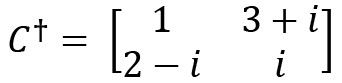
Just as we saw with the definition of a symmetric matrix, if , that is, the matrix is equal to its adjoint, then it is known as a Hermitian matrix.

Let's see how we can perform basic arithmetic operations on matrices such as addition and multiplication. Let's start with addition.

Matrix addition

Now, let's see how we can add two matrices. Let's define matrices A and B. Matrix addition is defined only for square matrices. We will look at a general case and then see an example:

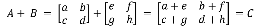
Our example for illustrating the addition of matrices is as follows:

and B , then

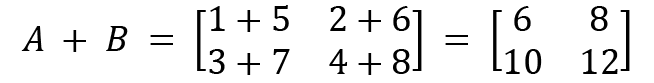
It can be observed that the corresponding elements are added together in matrix addition. The same method can be followed for matrix subtraction as well.

Let's see the properties of matrix addition. For A, B, and C matrices with size m x n, we have the following:

  • Commutative:
  • Associative:
  • Additive identity: , where O is a unique m x n matrix that, when added to A, gives back A
  • Additive inverse: , where
  • Transpose property:

Next, we will look at matrix multiplication.

Matrix multiplication

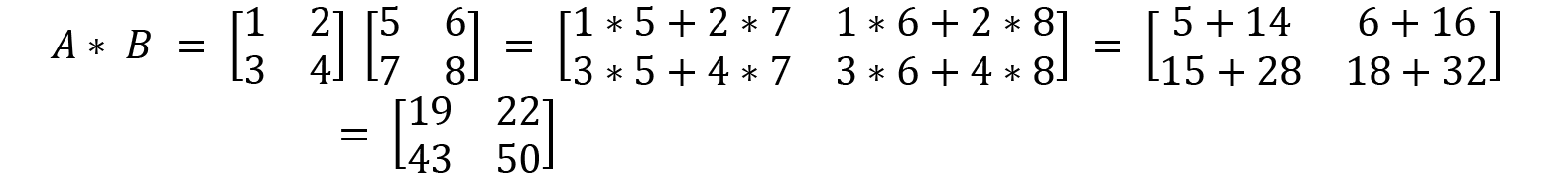
Let's look at the matrix multiplication process, which will later help us to understand multiple quantum gates applied to qubits in Chapter 2, Quantum Bits, Quantum Measurements, and Quantum Logic Gates. This is defined when the number of columns of the first matrix is equal to the number of rows of the second matrix. Let's take an example of a general case for matrix multiplication:

We take this example and multiply A and B together as shown here:

Now, if we define an operator and make it operate on the qubit , which is like , we can get . We see that remains unchanged by the operation of K. But if you apply , then you will get and you can verify it yourself! This means that the operator K changes the sign of the qubit only when it is in the state.

It is useful to remember that , and similarly, for complex matrices, . It will be a good exercise for you to prove that matrix multiplication is not commutative, which means that for any two matrices .

Let's see the properties of matrix multiplication. For A, B, and C matrices with size m x n, we have the following:

  • Associative:
  • Distributive:
  • Multiplicative identity:

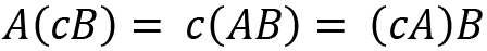
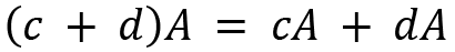
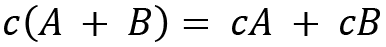
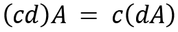
For two scalars c and d, a few properties on scalar multiplication are provided as follows:

We have now discussed some basic arithmetic operations on matrices. Now let's see how we can calculate the inverse of a matrix.

Inverse of a matrix

The inverse of a matrix represents the undoing of a transformation that has been done by a matrix. So, if the operator K transforms the vector space into some other space, then the inverse of K, denoted as , can be used to bring back the original vector space.

Let's see the calculation of an inverse of a 2x2 matrix. For a 2x2 matrix, the inverse is defined as follows: then .

If we take , then its inverse can be calculated as shown:

.

For an operator K, if , which means , then the operator is known as a unitary operator. I is the identity matrix whose diagonal entries are 1 and the rest are 0. The concept of a unitary operator and transformation are important because according to the postulate of quantum mechanics, time evolution in a quantum system is unitary. This means that these operators preserve the probabilities, and in a more mathematical sense, they preserve the length and angles of the vectors (quantum states). It is worth to note that eigenvalues of a unitary matrix is of a unit modulus.

Most of the time, a unitary matrix is denoted by U.

Some interesting properties of unitary matrices are as follows:

  • For any two complex vectors , the unitary preserves their inner product, so .
  • Since U commutes with its conjugate transpose (), it is called a normal matrix.
  • The columns of U form an orthonormal basis of .
  • The rows of U form an orthonormal basis of .
  • U is an invertible matrix with the property .
  • The eigenvectors of a unitary matrix are orthogonal.

Next, we will discuss the determinant and trace of a matrix and show how they can be calculated.

The determinant and trace of a matrix

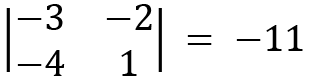
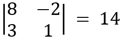
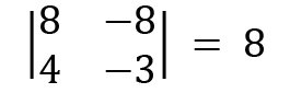
The determinant represents the volume of an n-dimensional parallelepiped formed by the columns of any matrix or an operator. The determinant is a function that takes a square matrix as an input gives a single number as an output. It tells us the linear transformation change for area or volume. For a 2x2 matrix, the determinant is calculated as follows:

then

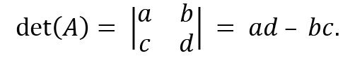
For a 3x3 matrix, the determinant is calculated like this:

then

It is worth pointing out that the determinant of a unitary matrix is 1, meaning . As an exercise, prove that the matrix is a unitary matrix with a determinant of 1.

The trace of a matrix or operator is defined as the sum of all the diagonal elements. This is given as follows:

If , then

An interesting property to note is that the trace of a matrix also represents the sum of the eigenvalues of the matrix and is a linear operation.

Let's now dive into the expectation value of an operator and its usefulness.

The expectation value (mean value) of an operator

Suppose we prepare a quantum state many times and we also measure an operator K each time when we prepare that state. This means we now have a lot of measurements with us, so it is natural for us to determine the cumulative effect of the measurement results. This can be done by taking the expected value of the operator K. This is given as follows:

So, the expected value is the average of all the measurement results, which are weighted by the likelihood values of the measurement occurring.

Now that we've learned about the various operations that can be performed on operators, let's learn about some important calculations that are performed on operators: eigenvalues and eigenvectors.

The eigenvalues and eigenvectors of an operator

Eigenvalues and eigenvectors are among the most important topics covered in linear algebra literature as they have a lot of significant applications in various fields. Apart from quantum computing, eigenvalues and eigenvectors find applications in machine learning (for instance, in dimensionality reduction, image compression, and signal processing), communication systems design, designing bridges in civil engineering, Google's Page Rank algorithm, and more.

Conceptually, we search for those vectors that do not change directions under a linear transformation but whose magnitude can change. This is essentially the concept of eigenvectors and eigenvalues. Just as we try to find roots of a polynomial, which are those values of a polynomial that restrict the shape of the polynomial, eigenvectors are those vectors that try to prevent a linear transformation from happening in the vector space, and eigenvalues represent the magnitude of those eigenvectors. Now, since we have an intuitive understanding of the concept, we can look at the more mathematical elements and the calculation.

A vector is called an eigenvector of an operator K if the following relation is satisfied:

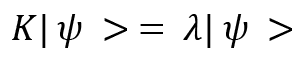
Here, is the eigenvector and is the associated eigenvalue, which is also a complex number. If the eigenvectors of an operator represent the computational basis, then any state can be written as the linear combination of the eigenvectors associated with the operator K. This is true for diagonal matrices, where there are only diagonal entries and the rest of the elements are zero. The inverse of a diagonal matrix is as simple as just taking a reciprocal value of the diagonal elements. This makes a lot of practical applications simpler.

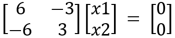
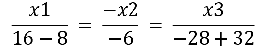
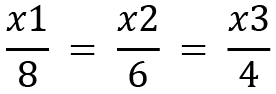
Now we will show the calculation process for eigenvalues and eigenvectors. Let's consider a 2x2 matrix; let's define a matrix A:

The characteristic equation for A that is used to calculate eigenvalues is given by the following:

We apply the values of A and the identity matrix:

Simplifying further, we will get the following:

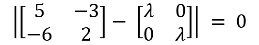
Now, subtracting from A, we have the following:

Now we will use the following relation to gain the characteristic equation of this matrix by calculating the determinant:
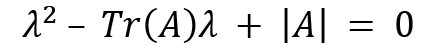
Here and , so we get the equation as follows:

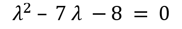
If we factorize the preceding characteristic equation, then we will get this:

These are the eigenvalues of the operatorA.

Now we will move on to calculating the eigenvectors. Let , and let's put this value into the following equation:

(

The equations can be formed as follows:

Since both the equations are the same, by simplifying and solving further, we will get the following:

Now we can choose a value for to have the eigenvectors. The simplest value is 1. Then, we will have the eigenvector . In a very similar process, ; you can verify it yourself.

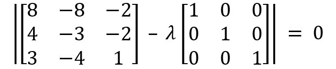
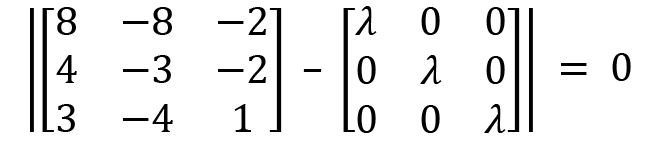
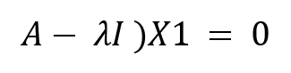
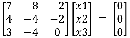
Let's now consider solving an example for a 3x3 matrix also. We will define a matrix called A:

The characteristic equation for A that is used for calculating eigenvalues is as follows:

We then apply the values of A and the identity matrix:

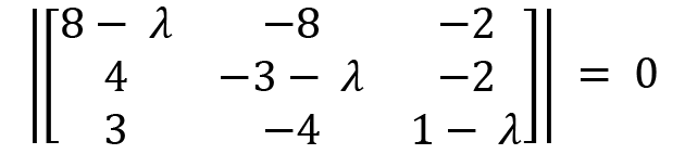
Simplifying a bit gives us the following:

Subtracting from A, we have this:

We will use a technique to simplify the calculations to calculate the determinant of this large matrix, which is as follows:

For calculating the minors, we just hide the rows and columns for the element for which we want to calculate the minor and then take the determinant of the remaining values.

Considering , we hide the first row and the first column, and the remaining elements become the following:

For 3, we hide the second row and the second column, and the remaining elements become this:

For 1, we get the following:

Therefore, the sum of the diagonal becomes . The trace of .

The final relation is this:

A calculator can be utilized to calculate the roots of this polynomial, and by doing so, you will get the roots of this cubic polynomial as follows:

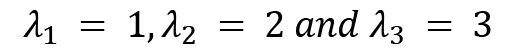
These are the eigenvalues of the operator A.

We will start by calculating the eigenvectors for A. We will start with and put this value in the following equation:

(

We will now utilize Cramer's rule to solve the preceding system of linear equations.

Consider any two rows or columns in the preceding matrix where adding or subtracting the values does not give 0 as an answer:

We can write as the numerators and then write the determinants as the respective denominators, where the entries are coefficients from the other variables. This can be done as follows:

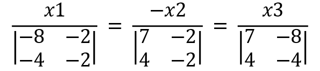
We observe that for , we take the coefficients of and as the determinant entries by hiding the terms. A similar process is done for others as well.

Solving the equation further, we will get the following result:

After solving a bit more, we have the following equation:

Therefore, the eigenvector , which can be simplified further to be .

Similarly, for .

We saw how to calculate the eigenvalues and eigenvectors of matrices/operators. Next, we are going to discuss an important concept known as tensor products.

Tensor products

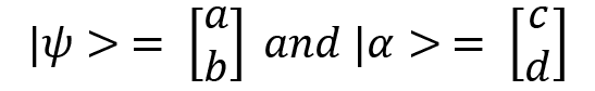
In quantum computing, we often have to deal with two, three, or multi-qubit systems instead of only one qubit. A two-qubit system would be , for example. Similarly, a three-qubit system would be . To deal with such composite systems, we use tensor products, which help us in performing various mathematical calculations on composite systems. The formal definition of a tensor product, as provided by An Introduction to Quantum Computing, is as follows:

The tensor product is a way of combining spaces, vectors or operators. An example is the union of two spaces H1 and H2 where each belongs to H, whose dimensions are n and m respectively. The tensor product of H1 H2 generates a new spacetime H of dimension nxm.

You can find the referenced text in the Further reading section.

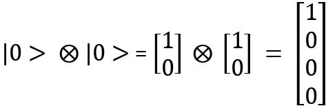
Let's now look at the calculation of tensor products for column vectors, which is the most common way of denoting a quantum state. Let's define two quantum states:

The tensor product of the two states is as follows:

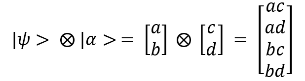
Using this, we can now describe the column vector representation of a two-qubit system. Suppose we consider . This can be written like this:

The tensor product has a distributive property, which is shown as follows:

.

For example, .

Proving all the properties of tensor products requires knowledge of abstract algebra and is out of the scope of this book. I highly recommend that you check out the books Finite-Dimensional Vector Space and Algebra by S. Lang (see the Further reading section) to gain a better understanding of the properties of tensor products.

The calculation of tensor products for two operators is given here. Let's define two 2x2 operators:

and

The tensor product of operators A and B is shown here:

Tensor products are very useful to verify the entanglement of quantum states. Entanglement is a useful property in quantum mechanics where two or more quantum systems can have some properties correlated with each other. As a consequence, knowing the properties of the first system can help to decipher the properties of the second system instantly.

With the conclusion of our discussion of tensor products, we also conclude our discussion of linear algebra. From the next section onward, we will discuss the visualization aspects of quantum computing, such as coordinate systems and complex numbers. We will also discuss probability theory in relation to quantum computing.


Coordinate systems, complex numbers, and probability

In this section, we will dive into three crucial topics of mathematics that are used heavily in quantum computation – coordinate systems, complex numbers, and probability. Coordinate systems are useful for the graphical representation of quantum states and to describe mathematical calculations in a visual format. After a fundamental understanding of coordinate systems, we will move on to complex numbers and look at their relationship with coordinate systems. You will see the simplicity of calculations carried out using the complex plane. Finally, we will learn about some fundamental probability theory concepts that are useful to quantum computing. Let's start with coordinate systems.

Introducing coordinate systems

In this section, you will learn about visualizing quantum states, which are just vectors in a mathematical sense. This will be useful for visualizing the geometry of quantum states and the various operations that you have already learned about in the previous sections. We will start with 2D coordinate systems and then move on to 3D coordinates before learning about the polar coordinate system.

2D Cartesian coordinate systems

Cartesian coordinates are one of the most useful graphical ways of visualizing 2D and 3D planes. Figure 1.1 shows the 2D coordinate system and displays the coordinates and vectors present in the space:

Figure 1.1 – A 2D Cartesian coordinate system

Figure 1.1 – A 2D Cartesian coordinate system

The coordinates in the Cartesian plane (Euclidean space) are denoted as (x,y), where the horizontal line is the x-axis and the vertical line is the y-axis; for example, in the preceding figure, three coordinates are represented as A = (2,3), B = (5,3), and C = (5,5). The point O = (0,0) is the origin. Using these coordinate values and the Pythagoras theorem for right triangles, the length AC can be calculated as . The distances in the Cartesian plane are called the Euclidean distance. This can be used to plot various kinds of functions, such as polynomial curves, circles, hyperbola, and exponentials. Cartesian coordinates can also be written in column vector form as .

We will now move on to 3D coordinate systems and understanding their usefulness.

3D Cartesian coordinate systems

In a 3D Cartesian system, we have 3 axes – the x-axis, the y-axis, and the z-axis. Often, we have to use 3D representations of vectors to understand the higher-dimensional aspect of quantum computing. Figure 1.2 shows the 3D coordinate system, and this coordinate system turns out to be very useful for understanding and visualizing higher-dimensional computations:

Figure 1.2 – A 3D Cartesian coordinates system

Figure 1.2 – A 3D Cartesian coordinates system

The coordinates can be denoted as (x,y,z). In this case, the x-axis is the tilted axis, the y-axis is the horizontal axis, and the z-axis represents the height or vertical axis. The mathematical calculations used for 2D systems can also be utilized for 3D systems. This 3D coordinate system will be very useful when we discuss Bloch sphere representations of qubits in Chapter 2, Quantum Bits, Quantum Measurements, and Quantum Logic Gates.

Next, we will introduce the polar coordinates system and discuss the conversion of coordinates between Cartesian and polar coordinate systems.

Converting Cartesian systems to polar coordinate systems

For simple calculations and complex numbers (covered in the next section), it is useful to convert Cartesian coordinates to polar coordinates, which involves using trigonometric functions. Polar coordinates are easily represented using a unit circle given in a 2D Cartesian plane. Figure 1.3 shows the polar coordinate system:

Figure 1.3 – Polar coordinate system

Figure 1.3 – Polar coordinate system

In a polar coordinate system, the (x,y) coordinates are represented as , where r is the radius and is given as and in degrees. To convert degrees into radians, multiply the degree value by . To convert radians back into degrees, multiply by . If you want to convert from polar to Cartesian, then you can use and . The polar representation that we learned about will be very useful for the calculations related to complex numbers.

Complex numbers and the complex plane

Jerome Cardan introduced the concept of complex numbers when it was found that while solving the roots of a quadratic polynomial, the square roots of negative numbers were encountered, which were not covered by real numbers. Due to this, the imaginary unit was introduced. This helped to write numbers such as

A complex number consists of real and imaginary parts. It is defined as follows:

Here, a and b are real numbers. In this, a is the real component and i b is the imaginary component, where b is the imaginary coefficient. Again, a complex number can be represented as a vector. In vector form, it z . In Figure 1.4, the complex number is shown:

Figure 1.4 – The Cartesian plane representing complex numbers

Figure 1.4 – The Cartesian plane representing complex numbers

In the preceding figure, you can see that the complex number has been represented in a Cartesian plane, where the x-axis denotes the real component and the y-axis denotes the imaginary component, more specifically, the imaginary coefficient, which is a real number.

Performing arithmetic operations on complex numbers is fairly intuitive and usually follows the normal algebraic rules.

For example, let's see the addition of two complex numbers:

The addition of complex numbers is commutative and associative, as follows:

  • Commutative: , for example,
  • Associative: , for example,

Subtraction is similar to addition. Let's see the multiplication of two complex numbers:

Similar to addition, multiplication has commutative and associative properties, along with another property called the distributive property. This is shown as follows:

  • Commutative: , for example,
  • Associative: , for example,
  • Distributive: , for example,

The complex conjugate of a complex number is given as follows:

The complex conjugate shows us the reflection of the complex number in another part of the axis provided in the complex plane.

The modulus of a complex number is very similar to calculating the magnitude of a vector and is given as follows:

We saw the polar coordinate system in the previous section and discussed how it is useful in the case of complex number representation. We will now look at using the polar coordinate system for complex number representation, which is a very important method to consider.

The main formula that connects polar coordinates with the complex plane is known as Euler's formula. The complex plane can be defined as a geometric visualization of the complex numbers in a 2D coordinate system, where the x-axis becomes the real part and the y-axis becomes the imaginary part. This is also known as the z-plane. Figure 1.5 shows the complex plane along with the Euler's relation, where (phi) is the angle:

Figure 1.5 – Euler's formula representation using a unit circle

Figure 1.5 – Euler's formula representation using a unit circle

Euler's formula is given as follows:

This formula helps connect the trigonometric relations with the complex exponentials. This helps us to represent a complex number in a polar representation. Let's define the complex number as follows:

Here, putting will give z as follows:

given as and in degrees.

If you calculate , you will see that it is always 1, and you can verify it yourself. It will require the usage of one of the most common trigonometric identities. Euler's identity is given as and is usually a good thing to know!

It is important to be familiar with some identities that make our mathematical calculations easier for the case of complex numbers. Two identities that are useful are these:

and

These identities are essentially representations of common trigonometric functions in terms of their complex exponentials.

The complex conjugate of is . The complex exponential form makes the calculations a lot easier.

Let's now dive into the topic of probability and learn about its significance in the field of quantum computing.

Probability

The concept of probability theory has always found significance in almost every area of science and technology, and quantum computing is no exception. Probability is a useful tool for dealing with the inherent randomness of real-life situations. In this section, we will dive into the basics of probability, random variables, and the usefulness of probability in quantum computing. Let's start with the definition of probability and its basic axioms.

Probability basics and axioms

Probability, as you might have guessed, is a branch of mathematics that deals with the likelihood or chance of events occurring. It is helpful in representing the likelihood of events happening in a system in terms of mathematical language. Girolamo Cardan wrote a book called Book on Games of Chance that introduced the first systematic treatment of the theory of probability.

Today, the applications of probability are huge in number because probabilistic techniques are used to predict the outcomes of various situations. It is used in games, weather forecasting, sports predictions, machine learning methods, reinforcement learning in artificial intelligence, deep learning, and quantum mechanics and physics for quantum measurement theory.

In quantum measurement theory, we check and calculate the probabilities of a quantum state being collapsed to a certain state. This is where the tools of probability theory are very useful. To make a probabilistic model of an unknown situation, two important things need to be considered: sample space and the law of probability.

Let's understand sample space first. A sample space is a set or collection of all the possible outcomes of a particular event. It is usually denoted by (pronounced as omega). For example, for an experiment of flipping a coin, we have a total of two possible outcomes, which are heads (H) and tails (T). So, the sample .

The law of probability assigns a numerical value (non-negative) to a particular event that represents the likelihood of that event occurring out of all the possible events. This is usually given as follows:

For example, the probability that tails can occur when we flip a coin is as follows:

P(T) =

Now we will look at some fundamental axioms of probability that are necessary for understanding the law of probability:

  • Probability can't be negative: This means that the probability of events from the sample space must be greater than or equal to zero. for every A.
  • Probability addition: For two disjointed events A and B, their probability of union is given by the sum of their individual probabilities. when P(A) and P(B) are independent events. If events are not independent, then .
  • The sum of all probabilities must be 1: The probability of the entire sample space must be equal to 1. P() = 1.

It is important to mention that , which is a complementary probability, and . Also, the probability values of a certain event A from the sample space must be so that the sum of all the probabilities of events present in the sample space adds up to 1. We observed that probabilities often have a numerical value, but many variables in the real world do not possess numerical values, so now we will discuss this issue in the next section by introducing random variables.

Discrete random variables and probability mass functions

Many times in the real world, the outcome of the events that we measure may not be numerical in nature. In those cases, random variables come to our rescue.

Random variables entail a mapping process that assigns a numerical value to the outcome of the events happening in a sample space. So, the random variable works as a function by taking outcomes from the sample space and giving them a numerical value taken in a real number line. In our case, we will be discussing discrete random variables.

Discrete random variables can be associated with a probability distribution, which is known as the Probability Mass Function (PMF). The PMF provides the probability of each of the numerical values that a discrete random variable can take. The sum of elements of the PMF always adds up to 1.

Let's consider a situation where a coin is flipped and every time heads comes up, you win $10, and every time tails comes up, you lose $10.

In random variable notation, this can be described as follows:

To describe the PMF for this coin flipping experiment, we have this:

Randomness, as we have seen, is a very useful phenomenon and has a wide variety of applications. In practical coding implementation, we have pseudo-random number generators that generate numbers between 0 and 1, but the process of generation is not truly random. This process is called sampling. One of the most useful benefits of a quantum computer would be to generate truly random numbers.

We will now focus our attention on calculating the mean and variance when data is provided to us.

Expectation (mean value) and variance calculation

The expectation is simply the mean of a random variable. It is the weighted mean of all the possible values of a random variable. The weights used for the purpose of expectation calculation are in proportion to the probabilities of the outcome of events. From the perspective of the PMF, the expected value of the PMF denotes the center of gravity of that PMF distribution. This is like calculating a linear combination of outcomes where the weights are the probabilities. Mean is also known as the first moment in statistics.

The formula that is used to calculate the expectation is as follows:

As an example, for a 6-sided die toss, we have the probability of each side as . Now, to calculate the expectation of this event, we need to multiply the probability by each of the numbered sides (the values of the outcomes), as shown here:

Variance is the measure of dispersion around the mean value. Intuitively, variance is about measuring the expected value of dispersion or the spread of the random variables from their mean value. Variance is also known as the second moment in statistics.

Therefore, the formula for variance becomes as follows:

Again, by considering the same 6-sided die example, we can calculate its variance as follows:

Essentially, variance defines the spread from the mean value, and in our case, the value is 2.92. In the next section, we will learn about the significance of the law of large numbers.

The law of large numbers

The law of large numbers states that the average or mean value of a large number of trials will be closer to the expected value and will tend to be closer and closer as the number of trials increases significantly.

In quantum computing, we perform measurements of probabilities of quantum states occurring after the quantum states are passed through a quantum circuit. This is done a number of times because the quantum computers that we have today are noisy and the quantum states that are prepared in the computer carry a lot of noise. So, to get accurate probability measurements, we run the measurements multiple times, and this is where the law of large numbers comes in. After a certain number of iterations of measurements, we start getting closer to the expected value, which is the ideal value.

With the conclusion of our discussion of probability, we also conclude our discussion of the essential mathematical concepts that are required for quantum computing. Let's now dive into the basics of algorithmic thinking and computer science that are essential for understanding quantum computing.


Defining computational thinking

The title of this book is Quantum Computing with Silq Programming, which means that quantum programming is at the heart of this book, and programming is a discipline that comes from computer science. Quantum computing is essentially a blend of many disciplines, including mathematics, quantum physics, quantum mechanics, and computer science. The concepts of quantum mechanics and physics will be introduced throughout the book as and when required. We have already covered the basic mathematics required for quantum computing, and now we are going to focus on another crucial aspect – computer science.

Computational thinking involves approaches to or methods of problem solving where we utilize ideas from computer science and express the problems and their solutions in such a way that the computer can execute them. This process involves breaking a large problem into smaller parts and then recognizing the pattern present in those small problems, finally developing a step-by-step solution to that problem. This is an efficient process to problem solving where once we convert a real-world complex problem so that a computer can understand it, a computer can then be used to solve the problem. This kind of thinking process is not only important to solve problems in science but is equally beneficial in other fields as well, such as social science, medical science, education, and business.

Computational thinking has four very important characteristics or skills associated with it:

  • Decomposition
  • Pattern recognition
  • Data representation and abstraction
  • Algorithmic design

In this section, we are going to discuss the first three skills, and then in the next section, we will discuss algorithms. Algorithms deserve a separate special section because they are a very significant aspect on their own, and covering them will later help us to understand various quantum algorithms. The algorithms covered here will be basic; discussing anything more advanced is beyond the scope of the book. In the next section, we will start our discussion of decomposition.

Decomposition

Decomposition is the first pillar of the computational thinking process. In the real world, problems are very complex to solve and require a lot of effort to reach a particular solution; therefore, it is much easier to divide a problem into smaller sub-problems and then work on them individually, because smaller ones are usually easier to solve. It may be that the smaller sub-problems are complex in themselves, and in that case, they can be divided into further smaller sub-problems. This process is also known as decomposition.

For example, suppose that you want to develop a mobile banking application so that offline transactions can be shifted completely to online. For this kind of problem, you can start by considering for which platform you would like to make your application, such as Android or iOS. Suppose you chose Android: you would then need to know some programming basics for Android as well. You will also be required to use Android tools to make the app. After all this, you might go about designing the app and its various functionalities step by step to complete the mobile banking application. That would all be a process of decomposition.

Now let's move on to pattern recognition and learn about its usefulness with regard to the computational thinking process.

Pattern recognition

Now we move on to another important pillar of the computational thinking process, pattern recognition. In the previous section, we discussed decomposition, where we divide a big problem into smaller sub-problems and then work on them. Often, we find some kind of pattern in the sub-problems that occurs frequently for most sub-problems. It's helpful to find this pattern to solve the sub-problems. Once we solve it once in one sub-problem, the rest becomes easy, because the same pattern is followed by other sub-problems as well. This then entails a repetitive process that can be followed until the problem is solved.

For example, consider the banking application we mentioned previously. Here, we want to include a feature where people can upload their photo and their proof of identity, and then the application will match the photo provided by the customer and the proof of identity to issue a bank passbook. This is where pattern recognition comes into the picture. The photo-matching technique consists of comparing the various pixels of the customer image with their proof of identity, and this process is repeated until a match of a person is accurately found. This is applied to a large number of customers in the bank who register for their banking application.

We have now looked at the first two pillars of computational thinking. Let's now move on to data representation and abstraction.

Data representation and abstraction

Now we will discuss the third component of the computational thinking process, that is, data representation and abstraction. When we are solving sub-problems, we will often find that some of the details are relevant to solving the problems and others are not. So, the process of data representation and abstraction involves the identification of those characteristics that are relevant to solving the problem and removing those characteristics that are not relevant. This process is also known as abstraction and is one of the most crucial elements in computer science and programming.

Considering the same bank application example, we can apply data representation and abstraction to the problem as explained. Every bank customer who registers for the banking application needs to provide some important details, such as their name, address, phone number, date of birth, income tax details, and email address. Now, in all of this data, there is a possibility that the name, date of birth, or address might be the same for two different customers. To differentiate customers, banks provide a unique account number to each of their customers to represent the data more efficiently so that registration can be performed easily. Also, data such as hobbies and food preferences does not hold any importance and can be filtered out.

There is another aspect of the computational thinking process that includes three characteristics – abstraction, automation, and analysis. These are very similar to the characteristics that we saw in the previous sections. Abstraction involves formulating the problem itself, such as constructing a banking application. Then, we move to automation, where the solution is expressed, such as coding various elements of the bank processes in the application using Android; and finally, we reach analysis, where the solution developed is executed on a computer and then evaluated for performance improvements.

The final pillar of computational thinking, algorithms, is discussed in the next section, as it is a significant part of computational thinking and programming.


Introducing computer algorithms

In the previous section, we discussed computational thinking and three of its primary pillars. The fourth and final pillar of computational thinking is algorithms. In this section, we will start with the definition of the linear search algorithm and see how it works. Then, we will discuss briefly the divide-and-conquer algorithms for searching. First, let's define what an algorithm is.

Defining an algorithm

An algorithm is a proper sequence of steps or rules that can be implemented in a computer to solve problems or perform calculations. It is like a recipe used to solve problems using computational thinking and is one of the most important parts of the computational process because this is where things start to get implemented in the real world. The algorithm is the very first step to writing a computer program!

Consider the example of making tea, which involves a sequence of steps that we need to follow in a certain order to make it successful. First of all, you will require the ingredients and resources, such as water, an electric kettle, a teabag, and a cup. Now we fill the kettle with water, switch it on, and let it boil. As soon as the kettle's boiled, we pour the water into the cup and then put the teabag into the cup. We let the teabag brew there for a few minutes and then we remove it. That's it – our tea is ready!

Now consider the steps for adding two numbers as performed by a computer. We know that for this, we would require the two numbers, and we will get an answer to our problem by the addition of the two numbers.

An algorithm for this would involve defining three variables that can store those two numbers and the answer. We would perform the addition and store the answer in the third variable. Finally, we could print the value of the third variable, which has the answer. You might wonder, can the tea-making job be done by a computer? And the answer is yes, it can! But the process is way more complex: for that, you have to teach a robot how to make tea! For a computer algorithm, we simply use the sequence of steps as instructions that are given to the computer to solve a particular problem.

Let's now learn about the way in which a linear search algorithm works. This is the most basic and simple of all the searching algorithms.

The linear search algorithm

Let's consider a searching problem where we have to search for a specific element in an array and return the index of the element when it is found. Some sample Python 3 code to do the searching is given as follows:

a = ['t','u','t','o','r','i','a','l']
x = 'o'
def linearsearch(a, x):
   for i in range(len(a)):
      if a[i] == x:
         return i
   return -1
print("element found at index "+str(linearsearch(a,x)))

The preceding code is used for a linear search operation. In linear searching, a user will provide a specific element to search in an array and the program will compare the value of the element with each of the values present in the array sequentially.

If you run the preceding code, you will get the output as element found at index 3. This is because indexing in Python starts at 0 and the a element is located at the sixth index. The input is the a element. You can clearly see in the code that each value present in the array is being compared with the input value provided. This means that the time of execution in this case linearly depends upon the length of the array.

There is another type of very famous algorithm called the divide-and-conquer algorithm, which represents the idea of computational thinking very well. It takes a bigger problem and then divides it into smaller sub-problems, solves each of those sub-problems individually, and then returns the solution, which is usually the solution to the whole problem. The most common example of a divide-and-conquer algorithm is the binary search algorithm, where the array is decomposed into parts and then searching is performed on the individual parts until the element is found.

Let's now learn about the complexity of algorithms and how we can make our algorithm implementations better in the next section.


The calculation of the time and space complexity of algorithms

In this section, we will introduce the concept of the time and space complexity of an algorithm, which helps us to measure the efficiency of an algorithm. This is important to measure because there are ways of optimizing algorithms for specific applications that are time-efficient but take up more memory. The time and space complexity will help us to analyze the performance of various algorithms and determine their use cases accordingly. We will then look at the notations that are used to calculate complexity, and finally, we will analyze and calculate the time and space complexity of a few algorithms.

Time and space complexity

Whenever we deal with algorithms, we are concerned with the speed and memory requirements of a computer program, because certain tasks require immediate real-time outputs. An example might be a self-driving car, where the camera gets real-time data from the road and then the computer processes it in real time to provide numerical outputs, which are fed into the computer controlling the car. The computer sends control signals carrying the information of the numerical outputs to the accelerator and brake sensors. For this reason, it becomes very important to calculate the complexity of any algorithm. Time is a crucial computational resource, and one that is very important to the design and optimization of algorithms.

The two complexities that we are concerned with are time and space complexity.

The time complexity of an algorithm is defined as the amount of time taken by an algorithm to execute some code in terms of the amount of input to the algorithm. This time is not an actual time in seconds, minutes, or hours; rather, it's the number of times an instruction is run by the computer. Space complexity is defined as the amount of memory (usually RAM) taken by the algorithm to execute some code in terms of the amount of input to the algorithm.

Let's dive into the mathematical notation used to calculate the time and space complexity of algorithms.

Notation for time and space complexity

We saw in the previous section the importance of time and space for a computer algorithm, and we saw an example of a linear search operation using Python.

For the calculation of the time and space complexity of algorithms, there are several asymptotic notations that are used to describe various aspects of the complexity of the algorithm. Let's see their definitions now.

  • Big O notation: For the asymptotic upper bound, we use the O (big O) notation.

    For a given function is defined as follows:

    : There exist positive constants c and such that for all }.

  • Big notation: For the asymptotic lower bound, we use the (big Omega) notation. Mathematically, it is defined very similarly to big O notation.

    For a given function is defined as follows:

    : There exist positive constants c and such that for all }.

  • Big notation: For the asymptotic tight bound, we use the (big Theta) notation.

    For a given function , is defined as follows:

    : There exist positive constants , and such that for all .

Since now we have covered the essential notations, let's look at the calculation and analysis of a few algorithms to give you an idea of the usage of these notations.

Calculation and analysis of the complexity of algorithms

For the analysis of algorithms, we mostly use big O notation to calculate the worst-case and average-case scenarios of algorithms. The upper bound given by big O notation is a very useful number to analyze the performance of the algorithm. For calculation of big O, we always ignore the lower-order terms and keep only the higher-order terms, because the lower-order terms become insignificant when the input given to a particular program is very high. Big O notation will focus on the number of steps a program took to complete the execution of a program or function.

For example, let's consider the case of linear search, which we discussed earlier. In that, you will observe that the loop will run for the length of the array, which means if there are N elements in the array, then the loop will run till element to search for the given input. This means the algorithm will take N steps to complete, and we write this as O(N). There is a possibility that the given input element will be found at the first index of the array itself. In that case, the algorithm took only a single step to find the element, and the complexity then becomes O(1). This means that O(1) is the best-case scenario and O(N) is the worst-case scenario.

However, as we discussed earlier, big O notation will generally be used to describe the worst-case scenarios of algorithms. It is also worth remembering that when the number of steps remains constant, the complexity is O(1), and this is true for reading, inserting, or deleting elements at the end of an array; it does not matter how many elements the array has.

We have described O(1) and O(N); there is another complexity called O(log N), and this is used with the binary search algorithm. Since in binary search we keep dividing the array into halves, for an N = 8 element array, it would only take N steps to find the element, meaning only 3 steps!

Let's now look at some practical code examples in Python 3, where we can calculate the time complexity of the algorithm. The first program we consider is for identifying a prime number:

def prime(n):
    for i in range(2, n):
        if n % i == 0:
            return False
    return True

If you consider the preceding code, you can see that the loop will run from 2 to the number that is provided as input by the user. This means that the number of steps taken by the code will be equal to the number given by the user. Therefore, the code has O(N) complexity. Also, an important point to consider is that big O notation throws away the constants, which means that O(50N) is equal to O(N).

This is because for some algorithms, it might be the case that ) is faster than O(50N) to a certain point, but after that point, O(50N) again becomes faster, so big O notation ignores the constants. This is true, for example, for distinguishing the sorting algorithms bubble sort and selection sort, where they both have ) complexity, but after a certain number of steps, selection sort becomes O(N) and remains like that no matter the size of the array. It is therefore natural to see that O(N) is faster than 0(N 2).

There are a lot of other cases as well where there are different time complexities, such as O(N*logN), O(N!) but they are out of the scope of this book. Computational complexity is a very broad discipline of computer science comprising various data structures and algorithms; proper analysis of all their time and space complexities would be difficult to cover in a short book. There are many good books and online courses on data structures and algorithms out there that discuss these concepts in a lot more detail.

The concepts and calculation of time and space complexity will be extremely useful when we discuss quantum algorithms and compare them with their classical versions in later chapters. For example, Grover's search algorithm will be discussed in Chapter 9, Quantum Algorithms III – Grover's Search Algorithm and Simon's Algorithm, where we will see that it takes ) time to find an element in an unsorted list!


Summary

In this chapter, we have covered plenty of fundamental concepts related to mathematics and computer science. We also looked at the relevance of mathematical concepts in relation to quantum computing, developing algorithmic thinking to aid us in understanding various quantum algorithms. Finally, you learned about the calculation of the time and space complexity of algorithms, which will allow you to compare the complexities of quantum algorithms with the classical algorithms you see in later chapters.

In the next chapter, we will look at the basics of quantum computing and learn about quantum measurements and single qubit quantum logic gates.


Further reading

  • Daniel Andrews, Big O: How to Calculate Time and Space Complexity, September 2019. https://www.inoutcode.com/concepts/big-o/.
  • Dr. Basant Agarwal, Benjamin Baka, Hands-On Data Structures and Algorithms with Python – Second Edition, Packt; Second edition, October 2018.
  • Dirac, P, (1939), A new notation for quantum mechanics. Mathematical Proceedings of the Cambridge Philosophical Society, 35(3), 416–418, doi:10.1017/S0305004100021162.
  • P. Kaye, I.Q.C.P. Kaye, P.K.R.L.M. Mosca, R. Laflamme, M. Mosca, and I.Q.C.M.Mosca, An Introduction to Quantum Computing, OUP Oxford, 2007
  • Paul R. Halmos, Finite-Dimensional Vector Spaces, First edition, Undergraduate Texts in Mathematics, Springer Publishing Company, Incorporated, 1993.
  • S. Lang, Algebra, Third edition, Graduate Texts in Mathematics 211, Springer-Verlag, 2002.
  • Grant Sanderson, 3Blue1Brown, https://www.youtube.com/playlist?list=PLZHQObOWTQDPD3MizzM2xVFitgF8hE_ab.
About the Authors
  • Srinjoy Ganguly

    Srinjoy Ganguly works as a quantum AI research scientist at Fractal Analytics. He has 4+ years of experience in quantum computing, and is an IBM Qiskit advocate and educator. He also teaches quantum computing at Woxsen University as a visiting professor. His research interests include QNLP, category theory with compositionality, variational quantum algorithms and their applications, and machine learning.

    Browse publications by this author
  • Thomas Cambier

    Thomas Cambier is a French programmer and software developer. After studying top-level mathematics, physics, and computer science at Ecole Polytechnique, France's leading engineering school, he obtained a Master's degree in computer science at ETH Zürich on a broad range of subjects going from algorithmics and cryptography to object-oriented programming. Deeply interested in the promising possibilities resulting from quantum computing, he wrote his Master's thesis on the design of quantum algorithms with Silq, a brand-new high-level quantum language created by a research group at ETH Zürich.

    Browse publications by this author
Quantum Computing with Silq Programming
Unlock this book and the full library FREE for 7 days
Start now