


In this introductory chapter, we will prepare all the necessary tools and data for the visual exploration of spatial phenomena, mapping, and analysis. After getting to know some basics about QGIS as a desktop GIS, you will learn how to install and configure it. Then, we will go through the most common spatial data sources and, in the end, aggregate them into a single spatial database that will be used for styling, mapping, and analysis in the following chapters.
In this chapter, we will go through the following topics:
QGIS installation
Graphical user interface (GUI), its elements, and its customization
Loading various types of spatial data from common sources
Projection's basics
Assembling data into a single spatial database
QGIS is a free and open source desktop GIS on which development began in 2002. Since 2007, the project has been developing under the umbrella of the Open Source Geospatial Foundation (OSGeo). A relatively young project, QGIS is gaining more and more popularity among individual users, private companies, and organizations all over the world due to the following reasons:
Distribution under the GNU General Public License (GPL), which guarantees users the freedom to use, study, share, and modify the software
Cross-platform support, which means that QGIS can run on Linux, Unix, Mac OS, Windows, and Android operating systems
Multiple vector and raster data format support, as well as database formats and functionalities
Permanent improvement of the core functionality, which encompasses data creation, editing, manipulation, analysis, storage, and visual representation
Permanent growth of the external functionality available from the so-called plugins supported by the international community of developers
Note
You can find more information about QGIS from its official website at http://qgis.org/ and its documentation chapter available at http://documentation.qgis.org/.
According to the release schedule of the QGIS project, a new version of QGIS is available every 4 months. Starting from QGIS 2.8, every third release has been a long-term release (LTR). It is maintained for a year, and then the next LTR occurs. Throughout this book, an LTR of QGIS 2.8 called "Wein" is used.
Installers for the current QGIS version are available for different operating systems from the download page of the official website at http://download.qgis.org. The 32-bit and 64-bit installation files for MS Windows are distributed as follows:
QGIS Standalone Installers: QGIS installation using these has no differences from the conventional software installation procedure under Windows
OSGeo4W Network Installer: Compared to standalone installers, this provides the following advantages:
Aside from QGIS, it allows us to install a large number of other packages to work with spatial data (command-line utilities, libraries, and desktop and server applications)
It ensures installation of the most up-to-date software versions being directly linked to constantly updating repositories
Once defined, the OSGeo4W working environment is convenient to use for automatic and timely updates, package addition, or package deletion
Let's go through the installation procedure of QGIS and its components with the OSGeo4W installer in the example of the latest 32-bit version. Since the installation (especially primary) requires downloading a large number of files, it is desirable to have a high-speed Internet connection. The installation procedure is as follows:
Download the latest version of the OSGeo4W 32-bit Network Installer, and double-click on
osgeo4w-setup-x86.exeto run the installation.In the installer window, select Advanced Install, as shown in the following screenshot. From now on, just read carefully and follow the instructions.

Choose Install from the Internet with the option to keep the downloaded files for future reuse.
Choose the directory for the OSGeo4W software suite installation.
C:\OSGeo4Wis a usual and convenient choice. If you want to use another directory, give it a proper name with a short path, excluding spaces and special symbols.Then, choose a directory to save the downloaded packages. You can create a new directory,
C:\OSGeo4W\Downloads, by typing in its name manually. Keep in mind that the volume of files to be downloaded is about 200 MB and you will need enough space to keep them all.Configure your Internet connection parameters, if any, and click on the Next button to proceed. After hitting the Next button, the list of all packages is downloaded and you enter the mode of package selection, as shown in the following screenshot. The available packages are grouped into the following categories: Commandline_Utilities, Desktop, Libs, and Web.

To install a package, click on the + sign to expand the category, and choose an application by clicking on the rounded arrow beside it (the word Skip will be replaced by the latest available version number).
To install the latest QGIS version, choose qgis: QGIS Desktop, and grass: GRASS GIS stable release. GRASS is a standalone GIS application that is closely integrated into QGIS and provides advanced geoprocessing functions.
After you've clicked on the Next button, the installer automatically detects the necessary dependencies and proceeds to download the packages and installation, as shown in the following screenshot:

After the installation completes, you will find the OSGeo4W group in the Start menu, with the following components:
MSYS: This is a set of GNU tools that ensure the creation of applications traditionally dependent on UNIX tools
OSGe4W Shell: This is a command-line interface for OSGeo4W utilities
QGIS Browser 2.8.1: This is a QGIS explorer used for navigation and data preview
QGIS Desktop 2.8.1: This is a QGIS desktop application
Setup: This is a OSGeo4W Installer launcher
GRASS GIS 7.0.0: This is GRASS GIS and its components
If you want to update QGIS or expand the current installation with some new components, simply click on the Setup shortcut from the OSGeo4W menu folder and run the Advanced installation procedure. The installer will check for available updates and necessary dependencies, download them, and install them.
When you first start QGIS, you will see the interface, as shown on the following screenshot. By definition, the QGIS interface uses the system language. For the purpose of this tutorial, you can change it in English by going to Settings | Options | Locale and restarting QGIS to apply your changes.

The QGIS interface consists of five main sections:
Menu bar: This provides access to all QGIS functions in the conventional form—drop-down menus.
Panels: These are windows that can be either docked or floating. By default, you can see two panels activated on the left side of the workspace.
The Layers panel is designated to display a tree view list of all loaded layers.
The Browser panel provides quick navigation and access to the various local, server, or online data sources. You can close or shrink a panel using special buttons in its top-right corner. You can also drag and drop it to a place handily.
Tip
Throughout this book, we will use the Browser panel from time to time, so try to assign it a proper position instead of closing it. For example, by dragging and dropping it onto the Layers panel, you can create two independent tabs: one for layers and the other for data source navigation. In this case, you will not have to sacrifice window the space necessary for expanding and viewing items.

Panels can be turned on or off by going to View | Panels. Similarly, you can right-click anywhere on the upper bar of the workspace, and a window with toggles will pop up. This window is divided by a horizontal line and the panels toggles are located in its upper part.
Toolbars: Menu functions are grouped into logical toolsets and placed as buttons in bars to provide handy access to all the necessary tools. By default, the following toolbars are turned on and displayed:

File toolbar

Map Navigation toolbar

Attributes toolbar

Digitizing toolbar

Label toolbar

Help and Plugins toolbars

Manage Layers toolbar
If you want to see a short tool reference, just hover your mouse pointer over the button and a yellow information window will pop up. Some buttons or toolbars are grayed out (for example, the Digitizing toolbar and Label toolbar), which means that they can be used only after some actions have been performed. For example, the Digitizing toolbar's buttons become available only after editing mode is activated for some layers. Toolbars are dockable and can easily be moved around the workspace. To move a toolbar, place the mouse arrow over its border marked by perforation dots. The arrow will turn into a cross, symbolizing that the toolbar can now be dragged and dropped to any other place while holding down the left button of the mouse. You can turn the toolbars on or off by navigating to View | Toolbars, or from the window called by a right click on any toolbar.
Map area: This is the largest section of the interface window, and is designed for data map display and visual exploration.
- Status bar: This briefly displays the following information about your current map overview: a progress bar of the rendering (visible only if rendering takes some time to show its progress), the mouse pointer's position coordinates, the scale, and the current coordinate reference system. It also contains toggles for switching from point position coordinates to extent, and temporarily turning off map rendering. There are also buttons used to open the coordinate reference system dialog
 and show the Log Message panel
  .
.
Advanced GUI customization is possible by navigating to Settings | Customization. From this dialog, you can get complete control over all menus, panels, bars, and widgets. To start the process of customization, turn on the Enable customization toggle. As long as you are not familiar with QGIS interface, it will be easier to enter  Switch to catching widgets in main application mode. In this mode, you can click on any GUI item you want to hide—a button on a toolbar or a toolbar itself. The chosen items are highlighted and the relevant customization tree item is expanded, as shown in the following screenshot. If you have chosen an item by mistake, simply click on it once again to unselect. Otherwise, you can expand the relevant item, check/uncheck some toggles, and click on OK. The changes are applied after QGIS restarts.

Tip
As your familiarity with QGIS grows and you start using it for different tasks, it might be convenient to create a few users' GUI profiles, aimed at different use cases (for example, digitizing, working with databases or raster data, and so on). To do so, you need to adjust all the necessary settings in the Customization dialog window, and save  them in a
 .ini file. After that, you will be able to quickly modify the interface just by loading settings  from a predefined customization file.
Some minor interface changes, such as general style, default icon size, font and more, are available from the Application group, which can be found by going to Settings | Options | General.
From the very beginning, QGIS has had a modular architecture that makes it easy to add new features or functions. Most functions in QGIS are implemented in so-called plugins, which are divided into the following types:
Core plugins: These are included in QGIS by default and are maintained by the development team. In order to be used, they should only be activated by a user.
External plugins: These are located in an external repository and are maintained by the authors. In order to be used, they should first be installed by a user. With time passing, some of the most useful and popular plugins are incorporated into the QGIS core functionality.
Plugin management implies their activation, installation, update, and removal, which are performed by navigating to Plugins | Manage and Install Plugins. There are several tabs in the dialog window. Clicking on an individual plugin in any of these tabs shows you detailed information: whether the plugin is experimental or not, the functionality, rating, author, version, and also some links to its homepage, code repository, and tracker:
All: Under this tab, you can see the full list of available plugins, both installed and not installed.
Installed: This tab shows the plugins that are already installed in QGIS. If you want to activate/deactivate a plugin, just check/uncheck the toggle beside it.
Not installed: This tab contains a list of all available plugins that are not installed in your QGIS.
The following tabs are not permanent and are shown only if there are plugins that satisfy some conditions:
Upgradeable: This tab is visible only when more recent versions of the installed plugins are available in the repositories.
Invalid: This tab is shown when there are installed plugins that are broken or incompatible with your QGIS version. If you click on an individual plugin from this tab, you will be shown the information about the possible cause of invalidity; so that you would be able to provide a consistent feedback to the developers.
New: This tab shows the not-installed plugins seen for the first time.

Settings: This tab allows you to define how often updates will be checked and whether to use experimental or deprecated plugins. While it is not recommended to use experimental plugins for production purposes, you can still activate the option to explore the entire range of available tools. By default, only QGIS Official Plugin Repository is connected, but you can connect additional repositories if you know them by clicking on the Add... button. For example, the previous screenshot shows how to add an external Boundless plugin repository.
To install a plugin, go back to the Not installed tab, select the plugin you want to install, and click on Install plugin. After that, the installation starts, and upon its completion, the message about successful installation is displayed. The installed plugin is activated by default and either appears in the Plugins menu, or is added to another relevant menu (for example, Vector or Raster). Also, some plugins appear as separate toolbars and panels that can be placed and turned on or off manually.
Finding and choosing a plugin that fits your needs might be difficult because their number is over 400 and is constantly growing. To explore the world of QGIS plugins, you can start from http://plugins.qgis.org/, which contains information about popular and featured plugins. If you are looking for a specific function but don't know the exact plugin name, we advise you to search by using tag words in the Manage and Install Plugins dialog window, as shown on the following screenshot:

The data in the GIS can be submitted as separate files, databases, or external online sources. Moreover, there are different data models used in the GIS to represent the geometry of spatial objects. The vector data model is mostly used to express discrete features, such as points (for example, separately growing trees and points of interest), lines (roads or railways), and polygons (buildings or administrative borders). Raster data is convenient for expressing continuous phenomena that are better represented by coverage than by points, lines, or polygons. The most common raster data sources are remote sensing imagery, digital elevation models, and scanned and georeferenced topographic maps.
QGIS uses the GDAL/OGR spatial data library to read and write multiple vector and raster file formats. In the following sections, we will briefly discuss the most common file formats that you can get your data in. Additionally, we will take a look at the recently widely used data sources, such as CSV files, files collected by GPS-receivers, and OpenStreetMap.
Most of our data is in the ESRI shapefile format, which is one of the most common vector data file formats. There are a few alternative ways of loading a shapefile into QGIS. You can open the dialog window by going to Layer | Add Layer | Add Vector Layer, or by clicking on the relevant button  on the Manage Layers toolbar, or by using the Ctrl + Shift + V keyboard shortcut.
In the Add vector layer dialog window, configure the following items:
Source type, which can be File, Directory, Database, or Protocol. By default, the File source type specified is suitable for loading spatial data represented by separate files, like in our case.
Consider the Encoding drop-down list options if the data you work with contains special symbols or the charset of its textual attributes differs from the conventional Latin symbology. In this case, you should choose an appropriate encoding type from the drop-down list. Our data does not contain any special symbols, so we accept the default System encoding.
The Browse button is meant for navigating to the work directory. There, you can choose one or several files (with the Ctrl key) to add after hitting the Open button.
Tip
For the first time, you are likely to be overwhelmed by the amount and diversity of the available files. This is because in the GIS, a dataset is usually represented by several files with different extensions. For example, an ESRI shapefile consists of at least 4 files (
.shp,.shx,.dbf, and.prj) that share the same name, and among them,.shpis what you should select to load the data into QGIS. You see all the files because the file type filter in the bottom-right corner of the window is set to All files by default. To hide all unnecessary files, choose the ESRI shapefiles file type. In future, don't forget to adjust the filter according to the desired file type.
Alternatively, you can use the Browser panel to navigate to the working directory. Select the files you want to load (either one or several, by holding down the Ctrl key), and then just drag and drop them onto the map area. If you want to simplify the navigation, add the folder you are currently working with to Favourites from its right-click menu shortcut.

The loaded files are assigned random colors. Don't worry about that as of now; we will cover layer symbology in Chapter 2, Visualizing and Styling the Data.
The procedure of adding raster files is similar to what was described earlier, so we will briefly go through it for the example of the common raster file format GeoTIFF:
-
You can load a raster file by going to Layer | Add Layer | Add Raster Layer, by clicking on the relevant button
 on the Manage Layers toolbar, or by using the Ctrl + Shift + R keyboard shortcut.
In the Open a GDAL Supported Raster Data Source window, go to the work directory.
To see available the GeoTIFF files, remember to adjust a file type filter, select one or more files (by holding down the Ctrl key), and click on Open. Alternatively, you can drag and drop rasters from the Browser panel.
ESRI Personal GeoDatabase is an original ArcGIS data format where all of the database's content is held in a single .mdb Microsoft Access file. It is widely used to store data in a single data file instead of multiple files of different formats.
Adding an ESRI file geodatabase to QGIS is similar to adding any other vector format:
-
Access the dialogue window by going to Layer | Add Layer | Add Vector Layer, or by clicking on the relevant button on the Manage Layers toolbar, or with the Ctrl + Shift + V keyboard shortcut.
Go to the work directory, set the file type filter to ESRI Personal GeoDatabase, and select the database file you want to import data from.
In the Select vector layers to add... window, you will see the available layers and their characteristics. Click on the layers to be added and hit OK.

Note
Raster layers contained in the database will be interpreted and loaded into QGIS as bounding-box polygons. If the data is stored in tables that do not contain any spatial features, the geometry type will be displayed as Unknown. The tables will be loaded and available for exporting to other formats (for example,
.dbf) or joining with spatial data layers.
A Comma-separated values (CSV) file is another popular data file format. In fact, it is just a spreadsheet with field values delimited by commas. There are various delimiters possible instead of commas (for example, tabs, spaces, colons and so on). Very often, these tables contain spatial data in the form of positional attributes represented by point longitude or latitude (XY) coordinates, or well-known text (WKT) geometry that describes points, lines, or polygons.
In our dataset, we have a CSV file called noise.csv. It contains the details of noise complaints registered mostly by the New York City Police Department. To add this file as a spatial layer, follow these steps:
-
Open the Create a Layer from a Delimited Text File dialog window by going to Layer | Add Layer | Add Delimited Text Layer, or just click on the relevant button
 in the Manage Layers toolbar.
After browsing and pointing to your file, QGIS tries to parse it using the specified delimiter. By default, the comma delimiter is used, but you can specify any other delimiter using Custom delimiters (comma, tab, space, and so on) or Regular expression delimiter.

The dialog also provides access to a number of other useful settings; for example, turning on First record has field names creates headers for fields. After defining the geometry as Point coordinates, X field and Y field containing Longitude and Latitude values will be loaded from the dataset automatically.
After you have clicked on OK, QGIS reads the data and might show a delimited text file error message similar to Errors in file full_path_to_the_file/filename.csv 100 records discarded due to missing geometry definitions. This means that some points do not contain geographic coordinates, and so they cannot be located properly. After closing the message window, you will be prompted to specify the Coordinate Reference System (CRS) for the layer.

As we can see from the Latitude and Longitude column values, point coordinates were originally registered by the receiving devices of the Global Position System (GPS) in decimal degrees. It is also known that GPS uses the WGS 84 CRS. This is why in the Coordinate Reference System Selector window, we enter the EPSG: 4326 code filter and specify WGS 84 under Geographic Coordinate Systems as the initial CRS. After clicking on OK, you will see that the data is rendered in the map canvas as points.
Note
QGIS uses CRS definitions based on the European Petroleum Search Group's (EPSG) Geodetic Parameter Dataset, which contains detailed structured descriptions of coordinate reference systems and transformations of global, regional, national, and local applications. The database of EPSG identifiers can be used to specify a CRS in QGIS. You can read more about the EPSG Geodetic Parameter Dataset at http://www.epsg-registry.org/.
As GPS receivers became portable and relatively cheap, GPS tracking became a ubiquitous and widely used technique of collecting data during a field survey, or simply tracking your own routes while running or cycling. Depending on the receiver's capabilities, in addition to spatial coordinates, a lot of information can be registered and written—for example, time, elevation, and so on. Registered information is stored in points that represent location changes (way, track, or route points), a planned route (if it exists), and a track of movement. There are numerous formats for storing GPS data. As primary data format, QGIS uses the standard interchange GPX (GPS eXchange) format.
We will load the nyc_marathon.gpx file from our dataset. You can load a .gpx file as a vector layer by going to Layer | Add Layer | Add Vector Layer, by clicking on the relevant button in the Manage Layers toolbar, or by using the Ctrl + Shift + V keyboard shortcut. Go to the data directory and apply the GPS eXchange format (GPX) file type filter. Select the file (or files) you want to add and click on Open. Alternatively, you can drag and drop files from the Browser panel.

As GPS data consists of points, routes, and tracks, the window pops up where you choose exactly which feature you want to open. You can select one or more features by clicking on a row and holding down the Ctrl key. If you are not sure exactly which feature you need, use Select All. Every feature type will be presented in a separate layer. By turning layers on and off, you can check whether they contain data or not; for example, the file we work with contains only tracks and track points. You can remove unnecessary empty layers by right-clicking on the layer contextual shortcut Remove.

OpenStreetMap (OSM) is a crowdsourcing project aimed at the development of an open map of the world. Worldwide, the OSM community uses high-resolution remote sensing imagery, GPS surveying, and local knowledge to make the map as accurate and detailed as possible. As the OSM data is licensed under Open Data Commons' Open Database License (ODbL), it has recently become a widely used source of spatial data. Understanding the importance of unrestricted access to spatial data, QGIS supports OSM, providing integrated access and support for its data.
The QGIS core functionality is available from the OpenStreetMap menu under Vector. Here, you can find all the required tools to download the data and export it into conventional spatial data formats, but if you are new to the QGIS and OSM data concepts, you may find the process tedious. This is why we recommend that you use external QuickOSM plugin capabilities to download the OSM data.
After installation as described in the Extending functionality through plugins section, the plugin's main functionality can be accessed by going to Web | QuickOSM | QuickOSM. The Quick query tab of the main window contains everything you need to perform a query and get the data into QGIS. First, define a key=value pair from the drop-down lists, or just type it in manually.
Note
It can be quite difficult to select the appropriate tags for the first time if you are not familiar with the OSM tagging system. Each tag is a key=value pair that describes some point, linear, or polygonal feature. The key describes a broad class (for example, amenities), while the value gives the details (bank, cinema, café, bicycle parking, and so on). Use the Help with key/value button to know more about tagging from the OSM wiki page at http://wiki.openstreetmap.org/wiki/Mapfeatures.
Then, set up the area of interest extent by location name, map canvas, or layer. If the layer drop-down list is inactive, click on the  button beside it to refresh it. In the Advanced section, you can turn on/off different geometry types. By default, all geometry types are turned on, so all the relevant points, lines, and polygons will be downloaded. Browse to the directory you want to save the data in. In the following screenshot, you can see the example of the QuickOSM query used to download bicycle parking point data.

Tip
If you are familiar with the Overpass API query language, you can click on Show query or the Query tab to modify the initial query.
After clicking on the Run query button, the shapefile with the data will be loaded into the map canvas.
Projections define how real-world objects on the curved surface of the earth will be flattened and projected on a map-like planar surface. Different data sources are usually created and distributed in different projections, depending on acquisition techniques and the scope of application. To be able to manipulate and analyze them properly in QGIS, it is important to understand how it interprets and manages information about projections.
QGIS supports about 2,700 CRS. They constitute a database, each item of which is described by an ESPG identifier, and a description line in the format of the PROJ.4 projection library. To store and read information about projection, QGIS uses its own format stored in .qpj files. There are two important points to keep in mind while working with projections: a data source projection and project projection—which are not always the same.
When you load your data into QGIS, it tries to automatically define information about the projection from the accompanying projection description file and set it to a newly added layer. You can check the layer's projection information in the Layer Properties dialog. To open it, double-click on the layer name in Layers panel, or use the right-click contextual shortcut Properties. Information about the projection is shown in the Coordinate reference system section of the General tab, like this:

There are numerous projection description file formats, and they mostly depend on the data format and origin. One of the most common among them is a .prj file. This file format sometimes provides information about the projection in a reduced form, and QGIS cannot define it properly. If information about the projection is absent or incomplete, you will see that the projection description is missing or looks like this: USER:100000 - * Generated CRS (+proj=etc.). It means that QGIS didn't find an appropriate projection within its own database and added it as a custom CRS. If you are sure that the projection is standard but QGIS fails to interpret it properly because of a reduced description, specify it manually. There are different ways to assess the Coordinate Reference System Selector dialog as follows:
-
Double-click on the layer name in Layers panel to open the Layer Properties dialog. Under the General tab, click on the Select CRS button
 to select the necessary CRS from the Coordinate reference system selector dialog window.
By going to Layer | Set CRS of Layer(s).
Using the Ctrl + Shift + C keyboard shortcut.
By right-clicking on the layer shortcut Set Layer CRS.
In the Coordinate reference system selector dialog, choose the necessary CRS from the list and click on OK. Note that you can use a filter by key words or the EPSG code to hide unnecessary projections. With time, often used projections will be added to the list of the recently used CRS.
Note
If QGIS doesn't define a projection for your data automatically and you are not sure about projection name and EPSG code, use the Prj2EPSG website at http://prj2epsg.org/. In this service, you just need to upload your .prj file, and well-known text projection information from it will be converted into standard EPSG code.
Note that specifying the projection manually from the Properties dialog is a temporary solution; it does not persist after closing a file and/or exiting QGIS. This means that whenever you are loading this file into QGIS, you will have to specify the projection again. If you are going to work with the file in other projects, it is better to use the Define Current Projection tool by going to Vector | Data Management Tools | Define Current Projection. In this dialog, you can choose a predefined spatial reference system from the Coordinate reference system Selector dialog or Import spatial reference system from existing layer with a known CRS. In both the cases, the existing .prj file will be overwritten by QGIS with all the necessary parameters, and you will not have to adjust the projection manually next time.

All of this is true when you import files from external sources. If you create a shapefile in QGIS, both .prj and .qpj files are created, so you don't need to define the projection manually. The files projection will be interpreted correctly in the other GIS applications that read it from .prj files.
You can also maintain QGIS behavior when loading or creating a new layer that has no CRS information by going to Settings | Options | CRS, where three alternatives of CRS for new layers are available:
Prompt for CRS: In this case, you will always be asked to manually specify the CRS for the layer.
Use project CRS: The data will be automatically assigned a CRS set for a project. This is a convenient choice if you are using files in the same projection, but if their projection differs from what is specified, you will not be able to see them.
Use default CRS displayed below: Conventionally, EPSG:4326 - WGS 84 is used, but you can specify your own choice.
Working with projections can be tricky, unless you recognize the difference between the specify and define projection options. It's all about assigning information about the projection properly, but when you specify it, the result is temporary within a current working session. Once you define a projection, it becomes permanent unless redefined again. In both cases, if you choose the wrong projection, you will not be able to see your data on the map (at least in the area where you expect it to be). Usually it is good practice to specify the projection at first, comparing your data to the correctly projected dataset. If everything is okay, define it to make projection assignment permanent.
When you load QGIS, its map canvas projection is, by default, set to EPSG:4326 – WGS 84. This behavior is defined by the global default projection, which can be changed by going to Settings | Options | CRS | Always start new projects with this CRS.
However, when you start adding data, projection identifier automatically changes to the projection of the first loaded layer. So, by default, project projection is defined by the first loaded layer. Data source projection and project projection are not always the same. If they are different, QGIS can apply the so-called on-the-fly transformation. This means that it reads the data projection, and if it differs, automatically aligns it with the project projection, applying the necessary transformations. There are a few ways to specify the projection for the project and enable on-the-fly transformation:
By going to Project | Project Properties | CRS.
-
Click on the Current CRS button on the Status bar, and activating Enable 'on the fly' CRS transformation in the Project properties | CRS window.
Go to Settings | Options | CRS | Default CRS for new projects. Activate either Automatically enable 'on the fly' reprojection if layers have different CRS or Enable 'on the fly' reprojection by default.
In the last way, the difference is very subtle and is mainly obvious when adding the first layer to the project. In the case of automatically enabled reprojection, the default map canvas CRS will be superseded by the first layer projection, and the following layers will be automatically adjusted to it too. In the case of reprojection by default, all layers will be reprojected into the project initial CRS (this is usually default global projection, unless you've changed it).
After on-the-fly transformation is enabled, you will see an OTF abbreviation near the current CRS on the status bar, and the icon will become solid.
If you want to quickly change the project CRS according to a specific layer in the Layers panel, right-click on a layer and choose the Set Project CRS from Layer shortcut.
Now that we have loaded all of the available data into QGIS, let's aggregate it into a single database. QGIS supports working with various database management systems and their spatial extensions (PostgreSQL/PostGIS, Oracle Spatial/GeoRaster, MSSQL Spatial, SQL Anywhere, and SQLite/SpatiaLite). Among them, PostGIS and SpatiaLite are the ones you have probably already heard about. Being common, these spatial databases are usually used for different purposes. PostGIS is an example of an enterprise solution used mostly on a server to provide spatial data maintenance and access for multiple users. SpatiaLite is a lightweight file database for personal use. Usage of SpatiaLite database has a number of advantages as follows:
All of the data is stored in a single, portable file, and you don't get overwhelmed by different file types (for example,
.shp,.dbf,.shx,.prj,.qpj, and so on)Shapefile limitations for size (up to 2 GB) and field name length (10 characters) can be omitted
Built-in spatial indices allow you to perform searches for large areas faster
This is a real relational database in a single format that allows you to use various spatial functions and SQL-based workflows
Perform the following steps to assemble your data into a single SpatiaLite database:
First of all, you need to create an empty spatial database to load your data into. You can do this from the Browser panel. Right-click on the SpatiaLite entry and choose the Create database shortcut. Specify the folder and a
.sqlitedatabase file name. You will get the The database has been created message. Now you can expand the entry and see your newly created empty database.-
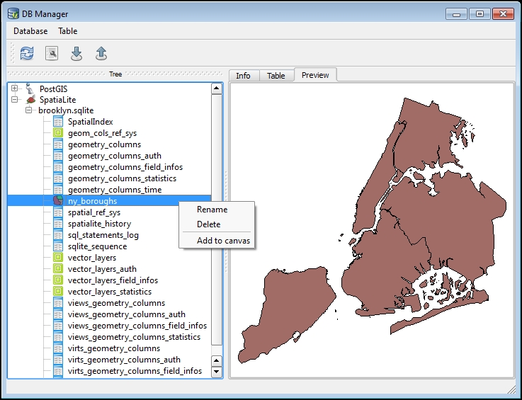
We will use the DB Manager core plugin that provides a single interface to work with different databases to load the data. The plugin functionality is accessible by going to Database | DB Manger. On the left side of the window, you can see a tree list of available database connections grouped by type. Once created, your database will automatically be available under the SpatiaLite item, and you can connect to it by double-clicking. When the connection is established, you will see general information about the database or its selected items in the Info tab on the right side of the window. To import files into the database, click on the Import layer/file button
 , or access it from the Table menu.

In the opened Import vector layer window, you should define the layer you want to import. It could be one of the already loaded layers available in the Input drop-down list, or the layer you choose from the filesystem by clicking on the browse button .... Then, define the Output table name (in our case, it is
ny_boroughs, the same as the input).
The following options allow you to exercise more control over your data:
Primary key: If this is not specified, the field will be named
pkby defaultGeometry column: If this is not specified, the field will be named
geomby defaultSource SRID and Target SRID: These are CRS EPSG codes read from the data, but you can specify them manually if the data isn't accompanied by projection files, or if you want to reproject it before loading it to the database
Encoding: If not specified, the dataset charset is set to UTF-8 by default
Drop existing table: If you import a table with the same name as a previously existing table, it will be replaced by the new table
Create single-part geometries instead of multipart: Multipart features will be disaggregated into single-part geometries before loading to the database
Create spatial index: A spatial index that allows faster spatial search and query performance will be created
After hitting OK and waiting a little (depending on the file size, the process may take some time), you will get the Import was successful message. To explore the imported table click on the Refresh button  , and you will see a geometry table in the list of database items. From the Info tab, you can view information about table, geometry type, fields, and triggers. The Table tab displays data in a tabular form, and the Preview tab displays spatial geometry, if any. By right-clicking on any element, you can delete, rename, or add it to the map canvas. All other opened layers can be loaded in a similar way.
For now, we have covered a few introductory topics and completed several tasks. First of all, you learned how to install QGIS, configure its interface, and extend functionalities with plugins. Then we discussed common data sources you can use to get data into QGIS. You are now capable of exploring and managing data in different projections. Last but not least, you imported all your data into a portable, lightweight SpatiaLite database file.
In the next chapter, we will move forward and reveal QGIS's potential for data visualization.

