


 Download code from GitHub
Getting Started with Parallel Computing and Python
The parallel and distributed computing models are based on the simultaneous use of different processing units for program execution. Although the distinction between parallel and distributed computing is very thin, one of the possible definitions associates the parallel calculation model with the shared memory calculation model, and the distributed calculation model with the message passing model.
From this point onward, we will use the term parallel computing to refer to both parallel and distributed calculation models.
The next sections provide an overview of parallel programming architectures and programming models. These concepts are useful for inexperienced programmers who are approaching parallel programming techniques for the first time. Moreover, it can be a basic reference for experienced programmers. The dual characterization of parallel systems is also presented. The first characterization is based on the system architecture, while the second characterization is based on parallel programming paradigms.
The chapter ends with a brief introduction to the Python programming language. The characteristics of the language, ease of use and learning, and the extensibility and richness of software libraries and applications make Python a valuable tool for any application, and also for parallel computing. The concepts of threads and processes are introduced in relation to their use in the language.
In this chapter, we will cover the following recipes:
- Why do we need parallel computing?
- Flynn's taxonomy
- Memory organization
- Parallel programming models
- Evaluating performance
- Introducing Python
- Python and parallel programming
- Introducing processes and threads
Why do we need parallel computing?
The growth in computing power made available by modern computers has resulted in us facing computational problems of increasing complexity in relatively short time frames. Until the early 2000s, complexity was dealt with by increasing the number of transistors as well as the clock frequency of single-processor systems, which reached peaks of 3.5-4 GHz. However, the increase in the number of transistors causes the exponential increase of the power dissipated by the processors themselves. In essence, there is, therefore, a physical limitation that prevents further improvement in the performance of single-processor systems.
For this reason, in recent years, microprocessor manufacturers have focused their attention on multi-core systems. These are based on a core of several physical processors that share the same memory, thus bypassing the problem of dissipated power described earlier. In recent years, quad-core and octa-core systems have also become standard on normal desktop and laptop configurations.
On the other hand, such a significant change in hardware has also resulted in an evolution of software structure, which has always been designed to be executed sequentially on a single processor. To take advantage of the greater computational resources made available by increasing the number of processors, the existing software must be redesigned in a form appropriate to the parallel structure of the CPU, so as to obtain greater efficiency through the simultaneous execution of the single units of several parts of the same program.
Flynn's taxonomy
Flynn's taxonomy is a system for classifying computer architectures. It is based on two main concepts:
- Instruction flow: A system with n CPU has n program counters and, therefore, n instructions flows. This corresponds to a program counter.
- Data flow: A program that calculates a function on a list of data has a data flow. The program that calculates the same function on several different lists of data has more data flows. This is made up of a set of operands.
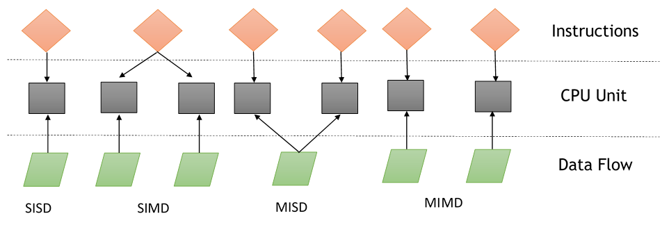
As the instruction and data flows are independent, there are four categories of parallel machines: Single Instruction Single Data (SISD), Single Instruction Multiple Data (SIMD), Multiple Instruction Single Data (MISD), and Multiple Instruction Multiple Data (MIMD):
Single Instruction Single Data (SISD)
The SISD computing system is like the von Neumann machine, which is a uniprocessor machine. As you can see in Flynn's taxonomy diagram, it executes a single instruction that operates on a single data stream. In SISD, machine instructions are processed sequentially.
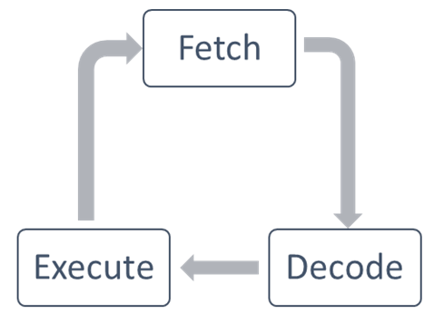
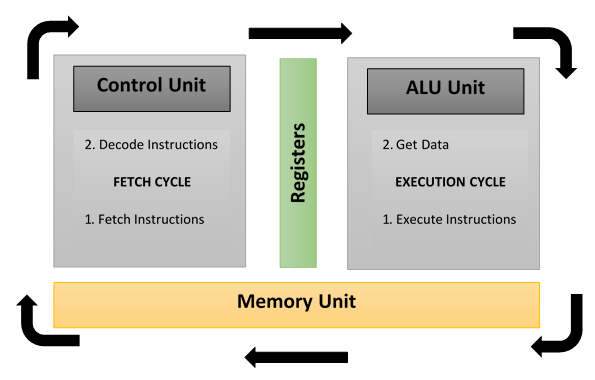
In a clock cycle, the CPU executes the following operations:
- Fetch: The CPU fetches the data and instructions from a memory area, which is called a register.
- Decode: The CPU decodes the instructions.
- Execute: The instruction is carried out on the data. The result of the operation is stored in another register.
Once the execution stage is complete, the CPU sets itself to begin another CPU cycle:
The algorithms that run on this type of computer are sequential (or serial) since they do not contain any parallelism. An example of a SISD computer is a hardware system with a single CPU.
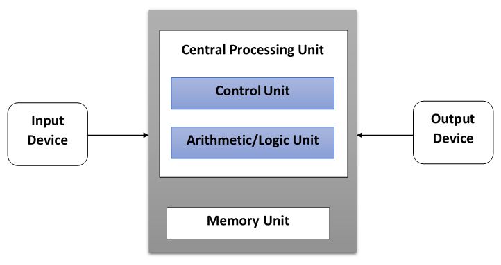
The main elements of these architectures (namely, von Neumann architectures) are as follows:
- Central memory unit: This is used to store both instructions and program data.
- CPU: This is used to get the instruction and/or data from the memory unit, which decodes the instructions and sequentially implements them.
- The I/O system: This refers to the input and output data of the program.
Conventional single-processor computers are classified as SISD systems:
The following diagram specifically shows which areas of a CPU are used in the stages of fetch, decode, and execute:
Multiple Instruction Single Data (MISD)
In this model, n processors, each with their own control unit, share a single memory unit. In each clock cycle, the data received from the memory is processed by all processors simultaneously, each in accordance with the instructions received from its control unit.
In this case, the parallelism (instruction-level parallelism) is obtained by performing several operations on the same piece of data. The types of problems that can be solved efficiently in these architectures are rather special, such as data encryption. For this reason, the MISD computer has not found space in the commercial sector. MISD computers are more of an intellectual exercise than a practical configuration.
Single Instruction Multiple Data (SIMD)
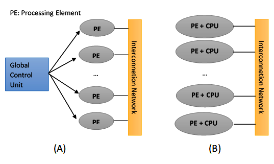
A SIMD computer consists of n identical processors, each with their own local memory, where it is possible to store data. All processors work under the control of a single instruction stream. In addition to this, there are n data streams, one for each processor. The processors work simultaneously on each step and execute the same instructions, but on different data elements. This is an example of data-level parallelism.
The SIMD architectures are much more versatile than MISD architectures. Numerous problems covering a wide range of applications can be solved by parallel algorithms on SIMD computers. Another interesting feature is that the algorithms for these computers are relatively easy to design, analyze, and implement. The limitation is that only the problems that can be divided into a number of subproblems (which are all identical, each of which will then be solved simultaneously through the same set of instructions) can be addressed with the SIMD computer.
With the supercomputer developed according to this paradigm, we must mention the Connection Machine (Thinking Machine, 1985) and MPP (NASA, 1983).
As we will see in Chapter 6, Distributed Python, and Chapter 7, Cloud Computing, the advent of modern graphics cards (GPUs), built with many SIMD-embedded units, has led to the more widespread use of this computational paradigm.
Multiple Instruction Multiple Data (MIMD)
This class of parallel computers is the most general and most powerful class, according to Flynn's classification. This contains n processors, n instruction streams, and n data streams. Each processor has its own control unit and local memory, which makes MIMD architectures more computationally powerful than SIMD architectures.
Each processor operates under the control of a flow of instructions issued by its own control unit. Therefore, the processors can potentially run different programs with different data, which allows them to solve subproblems that are different and can be a part of a single larger problem. In MIMD, the architecture is achieved with the help of the parallelism level with threads and/or processes. This also means that the processors usually operate asynchronously.
Nowadays, this architecture is applied to many PCs, supercomputers, and computer networks. However, there is a counter that you need to consider: asynchronous algorithms are difficult to design, analyze, and implement:
Flynn's taxonomy can be extended by considering that SIMD machines can be divided into two subgroups:
- Numerical supercomputers
- Vectorial machines
On the other hand, MIMD can be divided into machines that have a shared memory and those that have a distributed memory.
Indeed the next section focuses on this last aspect of the organization of the memory of MIMD machines.
Memory organization
Another aspect that we need to consider in order to evaluate parallel architectures is memory organization, or rather, the way in which data is accessed. No matter how fast the processing unit is, if memory cannot maintain and provide instructions and data at a sufficient speed, then there will be no improvement in performance.
The main problem that we need to overcome to make the response time of memory compatible with the speed of the processor is the memory cycle time, which is defined as the time that has elapsed between two successive operations. The cycle time of the processor is typically much shorter than the cycle time of memory.
When a processor initiates a transfer to or from memory, the processor's resources will remain occupied for the entire duration of the memory cycle; furthermore, during this period, no other device (for example, I/O controller, processor, or even the processor that made the request) will be able to use the memory due to the transfer in progress:
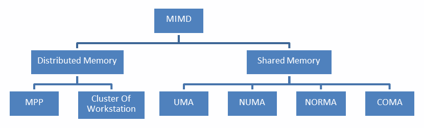
Solutions to the problem of memory access have resulted in a dichotomy of MIMD architectures. The first type of system, known as the shared memory system, has high virtual memory and all processors have equal access to data and instructions in this memory. The other type of system is the distributed memory model, wherein each processor has local memory that is not accessible to other processors.
What distinguishes memory shared by distributed memory is the management of memory access, which is performed by the processing unit; this distinction is very important for programmers because it determines how different parts of a parallel program must communicate.
In particular, a distributed memory machine must make copies of shared data in each local memory. These copies are created by sending a message containing the data to be shared from one processor to another. A drawback of this memory organization is that, sometimes, these messages can be very large and take a relatively long time to transfer, while in a shared memory system, there is no exchange of messages, and the main problem lies in synchronizing access to shared resources.
Shared memory
The schema of a shared memory multiprocessor system is shown in the following diagram. The physical connections here are quite simple:
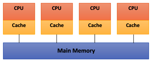
Here, the bus structure allows an arbitrary number of devices (CPU + Cache in the preceding diagram) that share the same channel (Main Memory, as shown in the preceding diagram). The bus protocols were originally designed to allow a single processor and one or more disks or tape controllers to communicate through the shared memory here.
The problem occurs when a processor modifies data stored in the memory system that is simultaneously used by other processors. The new value will pass from the processor cache that has been changed to the shared memory. Later, however, it must also be passed to all the other processors, so that they do not work with the obsolete value. This problem is known as the problem of cache coherency—a special case of the problem of memory consistency, which requires hardware implementations that can handle concurrency issues and synchronization, similar to that of thread programming.
The main features of shared memory systems are as follows:
- The memory is the same for all processors. For example, all the processors associated with the same data structure will work with the same logical memory addresses, thus accessing the same memory locations.
- The synchronization is obtained by reading the tasks of various processors and allowing the shared memory. In fact, the processors can only access one memory at a time.
- A shared memory location must not be changed from a task while another task accesses it.
- Sharing data between tasks is fast. The time required to communicate is the time that one of them takes to read a single location (depending on the speed of memory access).
The memory access in shared memory systems is as follows:
- Uniform Memory Access (UMA): The fundamental characteristic of this system is the access time to the memory that is constant for each processor and for any area of memory. For this reason, these systems are also called Symmetric Multiprocessors (SMPs). They are relatively simple to implement, but not very scalable. The coder is responsible for the management of the synchronization by inserting appropriate controls, semaphores, locks, and more in the program that manages resources.
- Non-Uniform Memory Access (NUMA): These architectures divide the memory into high-speed access area that is assigned to each processor, and also, a common area for the data exchange, with slower access. These systems are also called Distributed Shared Memory (DSM) systems. They are very scalable, but complex to develop.
- No Remote Memory Access (NoRMA): The memory is physically distributed among the processors (local memory). All local memories are private and can only access the local processor. The communication between the processors is through a communication protocol used for exchanging messages, which is known as the message-passing protocol.
- Cache-Only Memory Architecture (COMA): These systems are equipped with only cached memories. While analyzing NUMA architectures, it was noticed that this architecture kept the local copies of the data in the cache and that this data was stored as duplicates in the main memory. This architecture removes duplicates and keeps only the cached memories; the memory is physically distributed among the processors (local memory). All local memories are private and can only access the local processor. The communication between the processors is also through the message-passing protocol.
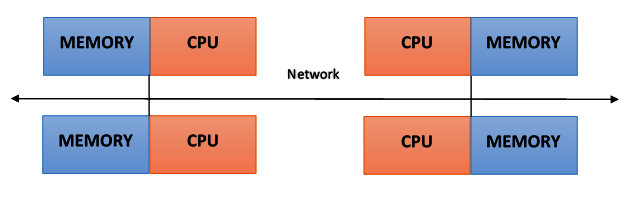
Distributed memory
In a system with distributed memory, the memory is associated with each processor and a processor is only able to address its own memory. Some authors refer to this type of system as a multicomputer, reflecting the fact that the elements of the system are, themselves, small and complete systems of a processor and memory, as you can see in the following diagram:
This kind of organization has several advantages:
- There are no conflicts at the level of the communication bus or switch. Each processor can use the full bandwidth of their own local memory without any interference from other processors.
- The lack of a common bus means that there is no intrinsic limit to the number of processors. The size of the system is only limited by the network used to connect the processors.
- There are no problems with cache coherency. Each processor is responsible for its own data and does not have to worry about upgrading any copies.
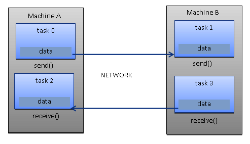
The main disadvantage is that communication between processors is more difficult to implement. If a processor requires data in the memory of another processor, then the two processors should not necessarily exchange messages via the message-passing protocol. This introduces two sources of slowdown: to build and send a message from one processor to another takes time, and also, any processor should be stopped in order to manage the messages received from other processors. A program designed to work on a distributed memory machine must be organized as a set of independent tasks that communicate via messages:
The main features of distributed memory systems are as follows:
- Memory is physically distributed between processors; each local memory is directly accessible only by its processor.
- Synchronization is achieved by moving data (even if it's just the message itself) between processors (communication).
- The subdivision of data in the local memories affects the performance of the machine—it is essential to make subdivisions accurate, so as to minimize the communication between the CPUs. In addition to this, the processor that coordinates these operations of decomposition and composition must effectively communicate with the processors that operate on the individual parts of data structures.
- The message-passing protocol is used so that the CPUs can communicate with each other through the exchange of data packets. The messages are discrete units of information, in the sense that they have a well-defined identity, so it is always possible to distinguish them from each other.
Massively Parallel Processing (MPP)
MPP machines are composed of hundreds of processors (which can be as large as hundreds of thousands of processors in some machines) that are connected by a communication network. The fastest computers in the world are based on these architectures; some examples of these architecture systems are Earth Simulator, Blue Gene, ASCI White, ASCI Red, and ASCI Purple and Red Storm.
Clusters of workstations
These processing systems are based on classical computers that are connected by communication networks. Computational clusters fall into this classification.
In a cluster architecture, we define a node as a single computing unit that takes part in the cluster. For the user, the cluster is fully transparent—all the hardware and software complexity is masked and data and applications are made accessible as if they were all from a single node.
Here, we've identified three types of clusters:
- Fail-over cluster: In this, the node's activity is continuously monitored, and when one stops working, another machine takes over the charge of those activities. The aim is to ensure a continuous service due to the redundancy of the architecture.
- Load balancing cluster: In this system, a job request is sent to the node that has less activity. This ensures that less time is taken to process the job.
- High-performance computing cluster: In this, each node is configured to provide extremely high performance. The process is also divided into multiple jobs on multiple nodes. The jobs are parallelized and will be distributed to different machines.
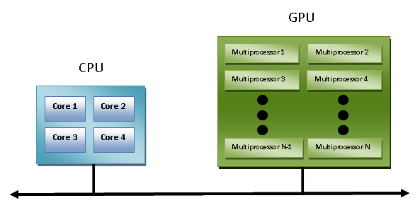
Heterogeneous architectures
The introduction of GPU accelerators in the homogeneous world of supercomputing has changed the nature of how supercomputers are both used and programmed now. Despite the high performance offered by GPUs, they cannot be considered as an autonomous processing unit as they should always be accompanied by a combination of CPUs. The programming paradigm, therefore, is very simple: the CPU takes control and computes in a serial manner, assigning tasks to the graphics accelerator that are, computationally, very expensive and have a high degree of parallelism.
The communication between a CPU and a GPU can take place, not only through the use of a high-speed bus but also through the sharing of a single area of memory for both physical or virtual memory. In fact, in the case where both the devices are not equipped with their own memory areas, it is possible to refer to a common memory area using the software libraries provided by the various programming models, such as CUDA and OpenCL.
These architectures are called heterogeneous architectures, wherein applications can create data structures in a single address space and send a job to the device hardware, which is appropriate for the resolution of the task. Several processing tasks can operate safely in the same regions to avoid data consistency problems, thanks to the atomic operations.
So, despite the fact that the CPU and GPU do not seem to work efficiently together, with the use of this new architecture, we can optimize their interaction with, and the performance of, parallel applications:
In the following section, we introduce the main parallel programming models.
Parallel programming models
Parallel programming models exist as an abstraction of hardware and memory architectures. In fact, these models are not specific and do not refer to any particular types of machines or memory architectures. They can be implemented (at least theoretically) on any kind of machines. Compared to the previous subdivisions, these programming models are made at a higher level and represent the way in which the software must be implemented to perform parallel computation. Each model has its own way of sharing information with other processors in order to access memory and divide the work.
In absolute terms, no one model is better than the other. Therefore, the best solution to be applied will depend very much on the problem that a programmer should address and resolve. The most widely used models for parallel programming are as follows:
- Shared memory model
- Multithread model
- Distributed memory/message passing model
- Data-parallel model
In this recipe, we will give you an overview of these models.
Shared memory model
In this model, tasks share a single memory area in which we can read and write asynchronously. There are mechanisms that allow the coder to control the access to the shared memory; for example, locks or semaphores. This model offers the advantage that the coder does not have to clarify the communication between tasks. An important disadvantage, in terms of performance, is that it becomes more difficult to understand and manage data locality. This refers to keeping data local to the processor that works on conserving memory access, cache refreshes, and bus traffic that occurs when multiple processors use the same data.
Multithread model
In this model, a process can have multiple flows of execution. For example, a sequential part is created and, subsequently, a series of tasks are created that can be executed in parallel. Usually, this type of model is used on shared memory architectures. So, it will be very important for us to manage the synchronization between threads, as they operate on shared memory, and the programmer must prevent multiple threads from updating the same locations at the same time.
The current-generation CPUs are multithreaded in software and hardware. POSIX (short for Portable Operating System Interface) threads are classic examples of the implementation of multithreading on software. Intel's Hyper-Threading technology implements multithreading on hardware by switching between two threads when one is stalled or waiting on I/O. Parallelism can be achieved from this model, even if the data alignment is nonlinear.
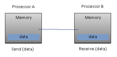
Message passing model
The message passing model is usually applied in cases where each processor has its own memory (distributed memory system). More tasks can reside on the same physical machine or on an arbitrary number of machines. The coder is responsible for determining the parallelism and data exchange that occurs through the messages, and it is necessary to request and call a library of functions within the code.
Some of the examples have been around since the 1980s, but only in the mid-1990s was a standardized model created, leading to a de facto standard called a Message Passing Interface (MPI).
The MPI model is clearly designed with distributed memory, but being models of parallel programming, a multiplatform model can also be used with a shared memory machine:
Data-parallel model
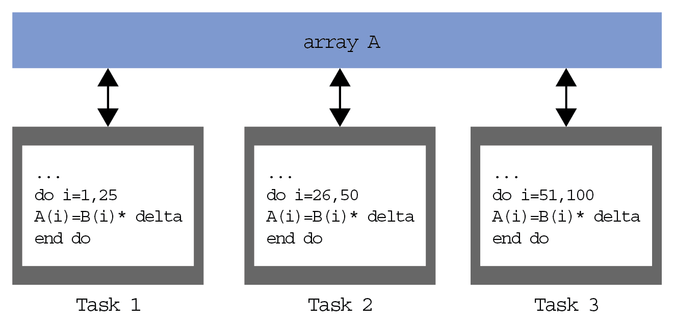
In this model, we have more tasks that operate on the same data structure, but each task operates on a different portion of data. In the shared memory architecture, all tasks have access to data through shared memory and distributed memory architectures, where the data structure is divided and resides in the local memory of each task.
To implement this model, a coder must develop a program that specifies the distribution and alignment of data; for example, the current-generation GPUs are highly operational only if data (Task 1, Task 2, Task 3) is aligned, as shown in the following diagram:
Evaluating the performance of a parallel program
The development of parallel programming created the need for performance metrics in order to decide whether its use is convenient or not. Indeed, the focus of parallel computing is to solve large problems in a relatively short period of time. The factors contributing to this objective are, for example, the type of hardware used, the degree of parallelism of the problem, and the parallel programming model adopted. To facilitate this, the analysis of basic concepts was introduced, which compares the parallel algorithm obtained from the original sequence.
The performance is achieved by analyzing and quantifying the number of threads and/or the number of processes used. To analyze this, let's introduce a few performance indexes:
- Speedup
- Efficiency
- Scaling
The limitations of parallel computation are introduced by Amdahl's law. To evaluate the degree of efficiency of the parallelization of a sequential algorithm, we have Gustafson's law.
Speedup
The speedup is the measure that displays the benefit of solving a problem in parallel. It is defined as the ratio of the time taken to solve a problem on a single processing element (Ts) to the time required to solve the same problem on p identical processing elements (Tp).
We denote speedup as follows:

We have a linear speedup, where if S=p, then it means that the speed of execution increases with the number of processors. Of course, this is an ideal case. While the speedup is absolute when Ts is the execution time of the best sequential algorithm, the speedup is relative when Ts is the execution time of the parallel algorithm for a single processor.
Let's recap these conditions:
- S = p is a linear or ideal speedup.
- S < p is a real speedup.
- S > p is a superlinear speedup.
Efficiency
In an ideal world, a parallel system with p processing elements can give us a speedup that is equal to p. However, this is very rarely achieved. Usually, some time is wasted in either idling or communicating. Efficiency is a measure of how much of the execution time a processing element puts toward doing useful work, given as a fraction of the time spent.
We denote it by E and can define it as follows:

The algorithms with linear speedup have a value of E = 1. In other cases, they have the value of E is less than 1. The three cases are identified as follows:
- When E = 1, it is a linear case.
- When E < 1, it is a real case.
- When E << 1, it is a problem that is parallelizable with low efficiency.
Scaling
Scaling is defined as the ability to be efficient on a parallel machine. It identifies the computing power (speed of execution) in proportion to the number of processors. By increasing the size of the problem and, at the same time, the number of processors, there will be no loss in terms of performance.
The scalable system, depending on the increments of the different factors, may maintain the same efficiency or improve it.
Amdahl's law
Amdahl's law is a widely used law that is used to design processors and parallel algorithms. It states that the maximum speedup that can be achieved is limited by the serial component of the program:

This means that, for example, if a program in which 90% of the code can be made parallel, but 10% must remain serial, then the maximum achievable speedup is 9, even for an infinite number of processors.
Gustafson's law
Gustafson's law states the following:

Here, as we indicated in the equation the following applies:
- P is the number of processors.
- S is the speedup factor.
- α is the non-parallelizable fraction of any parallel process.
Gustafson's law is in contrast to Amdahl's law, which, as we described, assumes that the overall workload of a program does not change with respect to the number of processors.
In fact, Gustafson's law suggests that programmers first set the time allowed for solving a problem in parallel and then based on that (that is time) to size the problem. Therefore, the faster the parallel system is, the greater the problems that can be solved over the same period of time.
The effect of Gustafson's law was to direct the objectives of computer research towards the selection or reformulation of problems in such a way that the solution of a larger problem would still be possible in the same amount of time. Furthermore, this law redefines the concept of efficiency as a need to reduce at least the sequential part of a program, despite the increase in workload.
Introducing Python
Python is a powerful, dynamic, and interpreted programming language that is used in a wide variety of applications. Some of its features are as follows:
- A clear and readable syntax.
- A very extensive standard library, where, through additional software modules, we can add data types, functions, and objects.
- Easy-to-learn rapid development and debugging. Developing Python code in Python can be up to 10 times faster than in C/C++ code. The code can also work as a prototype and then translated into C/C ++.
- Exception-based error handling.
- A strong introspection functionality.
- The richness of documentation and a software community.
Python can be seen as a glue language. Using Python, better applications can be developed because different kinds of coders can work together on a project. For example, when building a scientific application, C/C++ programmers can implement efficient numerical algorithms, while scientists on the same project can write Python programs that test and use those algorithms. Scientists don't have to learn a low-level programming language and C/C++ programmers don't need to understand the science involved.
You can read more about this from https://www.python.org/doc/essays/omg-darpa-mcc-position.
Let's take a look at some examples of very basic code to get an idea of the features of Python.
Help functions
The Python interpreter already provides a valid help system. If you want to know how to use an object, then just type help(object).
Let's see, for example, how to use the help function on integer 0:
>>> help(0)
Help on int object:

class int(object)
 | int(x=0) -> integer
 | int(x, base=10) -> integer
 |
 | Convert a number or string to an integer, or return 0 if no
 | arguments are given. If x is a number, return x.__int__(). For
 | floating point numbers, this truncates towards zero.
 |
 | If x is not a number or if base is given, then x must be a string,
 | bytes, or bytearray instance representing an integer literal in the
 | given base. The literal can be preceded by '+' or '-' and be
 | surrounded by whitespace. The base defaults to 10. Valid bases are 0
 | and 2-36.
 | Base 0 means to interpret the base from the string as an integer
 | literal.
>>> int('0b100', base=0)
The description of the int object is followed by a list of methods that are applicable to it. The first five methods are as follows:
 | Methods defined here:
 |
 | __abs__(self, /)
 | abs(self)
 |
 | __add__(self, value, /)
 | Return self+value.
 |
 | __and__(self, value, /)
 | Return self&value.
 |
 | __bool__(self, /)
 | self != 0
 |
 | __ceil__(...)
 | Ceiling of an Integral returns itself.
Also useful is dir(object), which lists the methods available for an object:
>>> dir(float)
['__abs__', '__add__', '__and__', '__bool__', '__ceil__', '__class__', '__delattr__', '__dir__', '__divmod__', '__doc__', '__eq__', '__float__', '__floor__', '__floordiv__', '__format__', '__ge__', '__getattribute__', '__getnewargs__', '__gt__', '__hash__', '__index__', '__init__', '__int__', '__invert__', '__le__', '__lshift__', '__lt__', '__mod__', '__mul__', '__ne__', '__neg__', '__new__', '__or__', '__pos__', '__pow__', '__radd__', '__rand__', '__rdivmod__', '__reduce__', '__reduce_ex__', '__repr__', '__rfloordiv__', '__rlshift__', '__rmod__', '__rmul__', '__ror__', '__round__', '__rpow__', '__rrshift__', '__rshift__', '__rsub__', '__rtruediv__', '__rxor__', '__setattr__', '__sizeof__', '__str__', '__sub__', '__subclasshook__', '__truediv__', '__trunc__', '__xor__', 'bit_length', 'conjugate', 'denominator', 'from_bytes', 'imag', 'numerator', 'real', 'to_bytes']
Finally, the relevant documentation for an object is provided by the .__doc__ function, as shown in the following example:
>>> abs.__doc__
'Return the absolute value of the argument.'
Syntax
Python doesn't adopt statement terminators, and code blocks are specified through indentation. Statements that expect an indentation level must end in a colon (:). This leads to the following:
- The Python code is clearer and more readable.
- The program structure always coincides with that of the indentation.
- The style of indentation is uniform in any listing.
Bad indentation can lead to errors.
The following example shows how to use the if construct:
print("first print")
if condition:
    print(“second print”)
print(“third print”)
In this example, we can see the following:
- The following statements: print("first print"), if condition:, print("third print") have the same indentation level and are always executed.
- After the if statement, there is a block of code with a higher indentation level, which includes the print ("second print") statement.
- If the condition of if is true, then the print ("second print") statement is executed.
- If the condition of if is false, then the print ("second print") statement is not executed.
It is, therefore, very important to pay attention to indentation because it is always evaluated in the program parsing process.
Comments
Comments start with the hash sign (#) and are on a single line:
# single line comment
Multi-line strings are used for multi-line comments:
""" first line of a multi-line comment
second line of a multi-line comment."""
Assignments
Assignments are made with the equals symbol (=). For equality tests, the same amount (==) is used. You can increase and decrease a value using the += and -= operators, followed by an addendum. This works with many types of data, including strings. You can assign and use multiple variables on the same line.
Some examples are as follows:
>>> variable = 3
>>> variable += 2
>>> variable
5
>>> variable -= 1
>>> variable
4

>>> _string_ = "Hello"
>>> _string_ += " Parallel Programming CookBook Second Edition!"
>>> print (_string_)
Hello Parallel Programming CookBook Second Edition!
Data types
The most significant structures in Python are lists, tuples, and dictionaries. Sets have been integrated into Python since version 2.5 (the previous versions are available in the sets library):
- Lists: These are similar to one-dimensional arrays, but you can create lists that contain other lists.
- Dictionaries: These are arrays that contain key pairs and values (hash tables).
- Tuples: These are immutable mono-dimensional objects.
Arrays can be of any type, so you can mix variables such as integers and strings into your lists, dictionaries and tuples.
The index of the first object in any type of array is always zero. Negative indexes are allowed and count from the end of the array; -1 indicates the last element of the array:
#let's play with lists
list_1 = [1, ["item_1", "item_1"], ("a", "tuple")]
list_2 = ["item_1", -10000, 5.01]

>>> list_1
[1, ['item_1', 'item_1'], ('a', 'tuple')]

>>> list_2
['item_1', -10000, 5.01]

>>> list_1[2]
('a', 'tuple')

>>>list_1[1][0]
['item_1', 'item_1']

>>> list_2[0]
item_1

>>> list_2[-1]
5.01

#build a dictionary
dictionary = {"Key 1": "item A", "Key 2": "item B", 3: 1000}
>>> dictionary
{'Key 1': 'item A', 'Key 2': 'item B', 3: 1000}

>>> dictionary["Key 1"]
item A

>>> dictionary["Key 2"]
-1

>>> dictionary[3]
1000
You can get an array range using the colon (:):
list_3 = ["Hello", "Ruvika", "how" , "are" , "you?"]
>>> list_3[0:6]
['Hello', 'Ruvika', 'how', 'are', 'you?']

>>> list_3[0:1]
['Hello']

>>> list_3[2:6]
['how', 'are', 'you?']
Strings
Python strings are indicated using either the single (') or double (") quotation mark and they are allowed to use one notation within a string delimited by the other:
>>> example = "she loves ' giancarlo"
>>> example
"she loves ' giancarlo"
On multiple lines, they are enclosed in triple (or three single) quotation marks (''' multi-line string '''):
>>> _string_='''I am a
multi-line
string'''
>>> _string_
'I am a \nmulti-line\nstring'
Python also supports Unicode; just use the u "This is a unicode string" syntax :
>>> ustring = u"I am unicode string"
>>> ustring
'I am unicode string'
To enter values in a string, type the % operator and a tuple. Then, each % operator is replaced by a tuple element, from left to right:
>>> print ("My name is %s !" % ('Mr. Wolf'))
My name is Mr. Wolf!
Flow control
Flow control instructions are if, for, and while.
In the next example, we check whether the number is positive, negative, or zero and display the result:
num = 1

if num > 0:
    print("Positive number")
elif num == 0:
    print("Zero")
else:
    print("Negative number")
The following code block finds the sum of all the numbers stored in a list, using a for loop:
numbers = [6, 6, 3, 8, -3, 2, 5, 44, 12]
sum = 0
for val in numbers:
    sum = sum+val
print("The sum is", sum)
We will execute the while loop to iterate the code until the condition result is true. We will use this loop over the for loop since we are unaware of the number of iterations that will result in the code. In this example, we use while to add natural numbers up to sum = 1+2+3+...+n:
n = 10
# initialize sum and counter
sum = 0
i = 1
while i <= n:
    sum = sum + i
    i = i+1 # update counter

# print the sum
print("The sum is", sum)
The outputs for the preceding three examples are as follows:
Positive number
The sum is 83
The sum is 55
>>>
Functions
Python functions are declared with the def keyword:
def my_function():
    print("this is a function")
To run a function, use the function name, followed by parentheses, as follows:
>>> my_function()
this is a function
Parameters must be specified after the function name, inside the parentheses:
def my_function(x):
    print(x * 1234)

>>> my_function(7)
8638
Multiple parameters must be separated with a comma:
def my_function(x,y):
    print(x*5+ 2*y)

>>> my_function(7,9)
53
Use the equals sign to define a default parameter. If you call the function without the parameter, then the default value will be used:
def my_function(x,y=10):
    print(x*5+ 2*y)

>>> my_function(1)
25

>>> my_function(1,100)
205
The parameters of a function can be of any type of data (such as string, number, list, and dictionary). Here, the following list, lcities, is used as a parameter for my_function:
def my_function(cities):
    for x in cities:
        print(x)

>>> lcities=["Napoli","Mumbai","Amsterdam"]
>>> my_function(lcities)
Napoli
Mumbai
Amsterdam
Use the return statement to return a value from a function:
def my_function(x,y):
    return x*y

>>> my_function(6,29)
174
Python supports an interesting syntax that allows you to define small, single-line functions on the fly. Derived from the Lisp programming language, these lambda functions can be used wherever a function is required.
An example of a lambda function, functionvar, is shown as follows:
# lambda definition equivalent to def f(x): return x + 1

functionvar = lambda x: x * 5
>>> print(functionvar(10))
50
Classes
Python supports multiple inheritances of classes. Conventionally (not a language rule), private variables and methods are declared by being preceded with two underscores (__). We can assign arbitrary attributes (properties) to the instances of a class, as shown in the following example:
class FirstClass:
    common_value = 10
    def __init__ (self):
        self.my_value = 100
    def my_func (self, arg1, arg2):
        return self.my_value*arg1*arg2

# Build a first instance
>>> first_instance = FirstClass()
>>> first_instance.my_func(1, 2)
200

# Build a second instance of FirstClass
>>> second_instance = FirstClass()

#check the common values for both the instances
>>> first_instance.common_value
10

>>> second_instance.common_value
10

#Change common_value for the first_instance
>>> first_instance.common_value = 1500
>>> first_instance.common_value
1500

#As you can note the common_value for second_instance is not changed
>>> second_instance.common_value
10


# SecondClass inherits from FirstClass.
# multiple inheritance is declared as follows:
# class SecondClass (FirstClass1, FirstClass2, FirstClassN)

class SecondClass (FirstClass):
    # The "self" argument is passed automatically
    # and refers to the class's instance
    def __init__ (self, arg1):
        self.my_value = 764
        print (arg1)

>>> first_instance = SecondClass ("hello PACKT!!!!")
hello PACKT!!!!

>>> first_instance.my_func (1, 2)
1528
Exceptions
Exceptions in Python are managed with try-except blocks (exception_name):
def one_function():
     try:
         # Division by zero causes one exception
         10/0
     except ZeroDivisionError:
         print("Oops, error.")
     else:
         # There was no exception, we can continue.
         pass
     finally:
         # This code is executed when the block
         # try..except is already executed and all exceptions
         # have been managed, even if a new one occurs
         # exception directly in the block.
         print("We finished.")

>>> one_function()
Oops, error.
We finished
Importing libraries
External libraries are imported with import [library name]. Alternatively, you can use the from [library name] import [function name] syntax to import a specific function. Here is an example:
import random
randomint = random.randint(1, 101)

>>> print(randomint)
65

from random import randint
randomint = random.randint(1, 102)

>>> print(randomint)
46
Managing files
To allow us to interact with the filesystem, Python provides us with the built-in open function. This function can be invoked to open a file and return an object file. The latter allows us to perform various operations on the file, such as reading and writing. When we have finished interacting with the file, we must finally remember to close it by using the file.close method:
>>> f = open ('test.txt', 'w') # open the file for writing
>>> f.write ('first line of file \ n') # write a line in file
>>> f.write ('second line of file \ n') # write another line in file
>>> f.close () # we close the file
>>> f = open ('test.txt') # reopen the file for reading
>>> content = f.read () # read all the contents of the file
>>> print (content)
first line of the file
second line of the file
>>> f.close () # close the file
List comprehensions
List comprehensions are a powerful tool for creating and manipulating lists. They consist of an expression that is followed by a for clause and then followed by zero, or more, if clauses. The syntax for list comprehensions is simply the following:
[expression for item in list]
Then, perform the following:
#list comprehensions using strings
>>> list_comprehension_1 = [ x for x in 'python parallel programming cookbook!' ]
>>> print( list_comprehension_1)

['p', 'y', 't', 'h', 'o', 'n', ' ', 'p', 'a', 'r', 'a', 'l', 'l', 'e', 'l', ' ', 'p', 'r', 'o', 'g', 'r', 'a', 'm', 'm', 'i', 'n', 'g', ' ', 'c', 'o', 'o', 'k', 'b', 'o', 'o', 'k', '!']

#list comprehensions using numbers
>>> l1 = [1,2,3,4,5,6,7,8,9,10]
>>> list_comprehension_2 = [ x*10 for x in l1 ]
>>> print( list_comprehension_2)

[10, 20, 30, 40, 50, 60, 70, 80, 90, 100]
Running Python scripts
To execute a Python script, simply invoke the Python interpreter followed by the script name, in this case, my_pythonscript.py. Or, if we are in a different working directory, then use its full address:
> python my_pythonscript.py
Installing Python packages using pip
pip is a tool that allows us to search, download, and install Python packages found on the Python Package Index, which is a repository that contains tens of thousands of packages written in Python. This also allows us to manage the packages we have already downloaded, allowing us to update or remove them.
Installing pip
pip is already included in Python versions ≥ 3.4 and ≥ 2.7.9. To check whether this tool is already installed, we can run the following command:
C:\>pip
If pip is already installed, then this command will show us the installed version.
Updating pip
It is also recommended to check that the pip version you are using is always up to date. To update it, we can use the following command:
C:\>pip install -U pip
Using pip
pip supports a series of commands that allow us, among other things, to search, download, install, update, and remove packages.
To install PACKAGE, just run the following command:
C:\>pip install PACKAGE
Introducing Python parallel programming
Python provides many libraries and frameworks that facilitate high-performance computations. However, doing parallel programming with Python can be quite insidious due to the Global Interpreter Lock (GIL).
In fact, the most widespread and widely used Python interpreter, CPython, is developed in the C programming language. The CPython interpreter needs GIL for thread-safe operations. The use of GIL implies that you will encounter a global lock when you attempt to access any Python objects contained within threads. And only one thread at a time can acquire the lock for a Python object or C API.
Fortunately, things are not so serious, because, outside the realm of GIL, we can freely use parallelism. This category includes all the topics that we will discuss in the next chapters, including multiprocessing, distributed computing, and GPU computing.
So, Python is not really multithreaded. But what is a thread? What is a process? In the following sections, we will introduce these two fundamental concepts and how they are addressed by the Python programming language.
Processes and threads
Threads can be compared to light processes, in the sense that they offer advantages similar to those of processes, without, however, requiring the typical communication techniques of processes. Threads allow you to divide the main control flow of a program into multiple concurrently running control streams. Processes, by contrast, have their own addressing space and their own resources. It follows that communication between parts of code running on different processes can only take place through appropriate management mechanisms, including pipes, code FIFO, mailboxes, shared memory areas, and message passing. Threads, on the other hand, allow the creation of concurrent parts of the program, in which each part can access the same address space, variables, and constants.
The following table summarizes the main differences between threads and processes:
| Threads |
Processes |
| Share memory. |
Do not share memory. |
|
Start/change are computationally less expensive. |
Start/change are computationally expensive. |
|
Require fewer resources (light processes). |
Require more computational resources. |
|
Need synchronization mechanisms to handle data correctly. |
No memory synchronization is required. |
After this brief introduction, we can finally show how processes and threads operate.
In particular, we want to compare the serial, multithread, and multiprocess execution times of the following function, do_something, which performs some basic calculations, including building a list of integers selected randomly (a do_something.py file):
import random

def do_something(count, out_list):
  for i in range(count):
    out_list.append(random.random())
Next, there is the serial (serial_test.py) implementation. Let's start with the relevant imports:
from do_something import *
import time
Note the importing of the module time, which will be used to evaluate the execution time, in this instance, and the serial implementation of the do_something function. size of the list to build is equal to 10000000, while the do_something function will be executed 10 times:
if __name__ == "__main__":
    start_time = time.time()
    size = 10000000
    n_exec = 10
    for i in range(0, exec):
        out_list = list()
        do_something(size, out_list)

    print ("List processing complete.")
    end_time = time.time()
    print("serial time=", end_time - start_time)
Next, we have the multithreaded implementation (multithreading_test.py).
Import the relevant libraries:
from do_something import *
import time
import threading
Note the import of the threading module in order to operate with the multithreading capabilities of Python.
Here, there is the multithreading execution of the do_something function. We will not comment in-depth on the instructions in the following code, as they will be discussed in more detail in Chapter 2, Thread-Based Parallelism.
However, it should be noted in this case, too, that the length of the list is obviously the same as in the serial case, size = 10000000, while the number of threads defined is 10, threads = 10, which is also the number of times the do_something function must be executed:
if __name__ == "__main__":
    start_time = time.time()
    size = 10000000
    threads = 10
    jobs = []
    for i in range(0, threads):
Note also the construction of the single thread, through the threading.Thread method:
out_list = list()
thread = threading.Thread(target=list_append(size,out_list))
jobs.append(thread)
The sequence of cycles in which we start executing threads and then stop them immediately afterwards is as follows:
    for j in jobs:
        j.start()
    for j in jobs:
        j.join()

    print ("List processing complete.")
    end_time = time.time()
    print("multithreading time=", end_time - start_time)
Finally, there is the multiprocessing implementation (multiprocessing_test.py).
We start by importing the necessary modules and, in particular, the multiprocessing library, whose features will be explained in-depth in Chapter 3, Process-Based Parallelism:
from do_something import *
import time
import multiprocessing
As in the previous cases, the length of the list to build, the size, and the execution number of the do_something function remain the same (procs = 10):
if __name__ == "__main__":
    start_time = time.time()
    size = 10000000
    procs = 10
    jobs = []
    for i in range(0, procs):
        out_list = list()
Here, the implementation of a single process through the multiprocessing.Process method call is affected as follows:
        process = multiprocessing.Process\
                  (target=do_something,args=(size,out_list))
        jobs.append(process)
Next, the sequence of cycles in which we start executing processes and then stop them immediately afterwards is executed as follows:
    for j in jobs:
        j.start()

    for j in jobs:
        j.join()

    print ("List processing complete.")
    end_time = time.time()
    print("multiprocesses time=", end_time - start_time)
Then, we open the command shell and run the three functions described previously.
Go to the folder where the functions have been copied and then type the following:
> python serial_test.py
The result, obtained on a machine with the following features—CPU Intel i7/8 GB of RAM, is as follows:
List processing complete.
serial time= 25.428767204284668
In the case of the multithreading implementation, we have the following:
> python multithreading_test.py
The output is as follows:
List processing complete.
multithreading time= 26.168917179107666
Finally, there is the multiprocessing implementation:
> python multiprocessing_test.py
Its result is as follows:
List processing complete.
multiprocesses time= 18.929869890213013
As can be seen, the results of the serial implementation (that is, using serial_test.py) are similar to those obtained with the implementation of multithreading (using multithreading_test.py) where the threads are essentially launched one after the other, giving precedence to the one over the other until the end, while we have benefits in terms of execution times using the Python multiprocessing capability (using multiprocessing_test.py).