


In this chapter, we will cover:
Building the Physical layer in the repository
Building the Business Model and Mapping layer
Adding multiple sources to the logical table source
Adding calculations to the fact table
Creating variables
Building the Presentation layer
Validating the repository using Consistency Check Manager
Uploading the repository
Oracle Business Intelligence Enterprise Edition Suite is a comprehensive reporting tool. The components of the suite are as follows:
This comprises the presentation of the business intelligence data to the clients through web browsers. This process communicates with the BI server component directly and consists of query clients such as Analysis Editor and dashboards. End users will be able to create and modify analyses or just access business data. According to the business requirements, customized analyses can be created and saved into the Presentation Catalog, which is a repository of Presentation Services. Then we can easily publish these reports using a dashboard.
Oracle BI Server is the main component in the suite. The BI server is simply a query engine that converts the logical requests to a physical SQL statement in order to execute it in the data sources. These optimized queries are generated based on the business rules that are defined in the BI server repository. These logical requests can be triggered from various applications. Obviously the most common one is Presentation Services, which belongs to the OBIEE components group. End users will be able to easily execute the logical requests from the dashboards. One single logical request can be used to query multiple physical data sources. Oracle BI Server and its metadata are transparent to the end users or to the person who executes a logical request. This conversion will be done based on metadata that should be configured by the BI developer. All of the business rules should be created as metadata.
This component manages the scheduled tasks. We are going to use either the Presentation Services or the Job Manager tool for creating scheduled tasks.
The metadata of the BI server is stored in the repository file on the server where the BI server service is running. A tool named BI Administration Tool that is installed with the default installation of OBIEE manages this repository.
In this chapter we're going to create this repository file from the beginning. Having a well-designed repository is crucial in business intelligence projects. We're going to use the Oracle database as a sample data warehouse.
The following are some samples of the data sources we'll also be using:
Relational databases
Multidimensional sources
Flat, XML, and CSV files
The repository is divided into three layers of metadata and are referred to as the following layers:
Physical layer
Business Model and Mapping layer
Presentation layer
We're going to start with the Physical layer.
The Physical layer defines the physical data sources and the Oracle BI Server uses these definitions in order to submit queries. The Physical layer is the first layer that we have to create. There could be many data sources based on different technologies and their metadata may exist in this layer.
We're going to use BI Administration Tool to create the repository and specify the business rules and object definitions. After we open BI Administration Tool, we are going to create a new repository from the File menu and save this new repository to its default location.

We'll have to specify the name of the new repository and its path. We can easily import the metadata with the wizard or skip importing the metadata at this moment. We're going to start the import process later on. So entering the password in Repository Password will be enough.

Clicking on No in the Import Metadata option will prompt the wizard to finish. Then it's going to show the content of the repository. We're going to see only three layers without any object definition.

These values should be entered in the Import Metadata - Select Data Source window:
Connection Type: The type of the data source should be defined in this field. One of the technologies should be selected from the drop-down list. We're going to use Oracle Database 11g R2 Version in our scenario, so the type is
OCI 10g/11gfor Oracle.Data Source Name: This is the name that is configured in the
tnsnames.orafile. By default, this file is located in the$ORACLE_HOME/network/admindirectory.User Name and Password: The last parameters are the username and the password of the user who has access to the tables.

The type of the metadata objects should be selected in the Select Metadata Types window. Then we're going to select the tables that we're interested in, in our BI project. So only four tables from
Supplier2schema are selected. We can easily import new tables when needed. Additionally, constraint definitions are also retrieved during the metadata import process.
After the wizard ends, we'll see that the database object definition is created and one Connection Pool object is created as well. It's the definition of the connection to the physical data source. We'll also notice that four of the table definitions are imported under the schema of
Supplier2. Now alias object definitions are going to be created. They are the objects representing the physical tables. Referencing to the same table twice in the same SQL statement causes circularity, and this situation is not allowed in the OBI repository. In order to avoid circular joins, alias object definitions are needed. Right after the import wizard ends, alias object definitions should be created by the developer manually. We'll right-click on the table and navigate to New Object | Alias from the menu list.
Actually, there are not any foreign key constraints defined on the tables in the database. In these kinds of cases, the primary key and foreign key relationship should be defined in the BI repository by creating joins. In order to create joins, select all aliases and right-click on them to open the Physical Diagram. Right after it, we'll use the New Join button to create the joins between the tables. It's going to ask about the columns that will be used in the join definition.

The definition of each join object looks like the one in the following screenshot. There's no information about the type of join in the Physical layer. So the join type will be set in the Business Model and Mapping layer. We should only specify the column mappings from the fact table to the dimension tables one by one. The foreign key columns in the fact tables will be referencing to the primary key columns in the dimension tables.

Now we've finished the basic tasks of the Physical layer. Physical tables and their aliases are created and also all the relationships between the tables are defined. We can say that creating the Physical layer is easier than the BMM layer. Most of the tasks are done by using wizards that take less time. The objects that are in the Business Model and Mapping layer are going to reference to the Physical layer objects. Obviously, having a well-designed Physical layer will make the other tasks in the BMM layer easier. When any report is executed at Presentation Services, the logical SQL statement is going to be generated based on the definitions in the BMM layer. Then this logical SQL statement is going to be converted to a physical SQL statement that is going to be executed at the database.
We only used some tables in our sample scenario. Actually, the Physical layer objects are dependent on the data sources. Let's imagine that if multiple databases, Excel spreadsheets, XML files, or multidimensional data sources exist, then all of them should be defined in the Physical layer. We're going to focus on multidimensional data sources in Chapter 4, Working with Multidimensional Data Sources.
The Business Model and Mapping layer defines the logical model of the data that maps the business rules to the Physical layer objects. There can be many business models that can be mapped with different kinds of data sources based on different technologies. Also dimensional modeling should be done in this layer. This can be achieved by creating dimension objects and their hierarchies. Also all about the calculation and aggregation rules will be defined in this layer.
As a summary, all the business rules are going to be created in this layer. It's probably the most important layer in the repository, and it'll definitely take longer to create the objects in this layer.
Creating business models can be done by two methods, manually or by drag-and-drop. If the manual object creation method is preferred, we'll have to create objects in the following order:
Create the business model.
Create the logical tables and map them to the physical tables.
Create the logical columns.
Define the logical joins.
Create the business model manually by right-clicking on the BMM layer and selecting New Business Model. (Give it a name, in this case
Sales.)Ensure that the Disabled option is checked because there's no other object in this business model. We're going to change this setting later.

After creating a blank and disabled business model, drag-and-drop the physical objects from the Physical layer onto the business model named
Sales.Automatically created objects are:
Logical dimension and fact tables
Logical columns and their mappings to Physical layer
Logical table sources for the dimension and fact tables
Logical keys and joins (can be accessed from the Business Model Diagram window)
Now it'll be good to make a clean-up because with this automated process all of the columns from the Physical layer are created as logical columns. Most probably we won't need all of the logical columns; we can easily delete the logical columns that are not required by right-clicking on the columns. Another task is renaming the logical tables and columns with meaningful names.

After making the clean-up, we'll see that some columns are deleted and some are renamed.

When we open the properties of the logical table source named
Fact_Orders, we'll find mappings from the Logical Column to the Physical column. Also if you need to access other details of the logical table source, you'll have to extend the logical table sources folder, so you'll find the logical table source definition.
The new business model is almost ready but still there is a missing step that is the aggregation rule for the columns in the fact table. By default, it's not set. The following are the options for the aggregation rule, so depending on the requirement you can use one of them:
SumandAvgCountandCount DistinctMaxandMinStdDevand so on
In order to set the aggregation rule for one logical column in the BMM layer, you'll have to open the properties window of that column and go to the Aggregation tab. You'll find the rules in the drop-down list and select one of them. The most common one will be
Sum. So we'll useSumas the aggregation rule in this demonstration. In the case of business requirements, we can use different aggregation rules. If you need to display the number of the rows, we can useCountas the aggregation rule.
So we've configured all of the measures in the fact table with the
Sumaggregation rule.
We created a simple business model in this section. Each logical table should have at least one logical table source. We might create multiple logical table sources as well, just in order to use summary tables or horizontal/vertical data federation. The important point in this layer is creating the logical joins. The Oracle BI Server will recognize the logical fact and dimension tables by checking the logical joins. Obviously, the logical joins are dependent on the physical joins, but we may have only one table in the Physical layer. So there won't be any physical join. Even in a single table scenario, we'll need to create fact and dimension tables in the BMM layer and create logical joins between them. At the end, all the objects will be referencing to only one single table. After working on the Business Model Diagram, we selected the aggregation rules that will be applied on the measure columns such as Sum, Count, and Avg. Is this a required step? Actually, it's not required. If you don't set the aggregation rule of the measures, you won't be able to see aggregated data in the reports. Let's assume that if the fact table contains one million rows, you'll see one million rows in the report. Although setting the aggregation rule is not a must, it's highly recommended to do it.
Regarding the business model, there is one more object type called logical dimensions. The Drill Down feature and aggregate (summary) tables can be used after dimensions are created. As you see, two important features are dependent on dimensions. We're going to focus on logical dimensions and their types in Chapter 2, Working with Logical Dimensions.
Because of the data warehouse design, data may be stored in the physical tables in the normalized way. That means some columns are stored in different tables. This kind of design is called as the snowflake schema. For example, let's assume that the product data is spread into different physical tables, for example, the price information doesn't exist in the product table and it's stored in the price list table. Another example is that supplier data can be stored in another table such as the suppliers table.
When this is the case, there's a business solution in Oracle Business Intelligence. We can add multiple sources to existing logical table sources.
In order to add multiple sources, we'll need to extend the existing repository and import these additional tables to the Physical layer. We're going to avoid using the physical tables directly, so we will create aliases for these new tables. You can see that they are already imported and aliases are created. Additionally, physical joins should be created.

Now we have to reflect these changes to the BMM layer. Although the new physical table definitions are created, the BMM layer is not aware of this information. Again there are two methods of making logical changes in the Business Model and Mapping layer, manually or drag-and-drop. We're going to drag-and-drop the new physical columns on to the logical table source (not on to the logical table).
When you drag the two columns named
PRICEandITEMSUPPLIERfrom the Physical layer on to the logical table source, you'll see that two new logical columns are added into theDim-Productlogical table.
After this action, there will be a modification in the logical table source. Normally, the logical table sources are mapped to a single physical table. But now you'll notice at the end of this action that the
Dim_PriceListandDim_Supplierphysical tables are also mapped with that logical table source. By default, it uses the Inner join type and we can change it based on the requirement analysis.
Another change in Logical Table Source is Column Mapping. It also automatically maps the new logical columns with the physical columns.

We added multiple sources into the logical table sources in this recipe. We could use the manual method, which would cost more time and steps, so we used the drag-and-drop method. If the supplier and price columns are used in the report the BI server is going to retrieve the data from the two different tables. This processing relies on the settings of the column mappings. Whenever a report is executed, the BI server is going to check the logical table sources and the column mappings. All logical columns should be mapped with the physical columns, otherwise the consistency check tool will generate an error.
Designing of the business model is a crucial step. Any mistake at this layer will cause generation of inaccurate result sets. When we start to construct the reports at Presentation Services, the logical SQL statement is going to be generated, based on the business rules in the model. It'll check the logical relationships, column mappings, aggregation rules of the measures, and so on.
We only created one business model in our scenario that doesn't contain any dimensions or multiple logical table sources. The business models are referenced by subject areas from the Presentation layer. They focus on a particular business view. We might create more business models according to the business requirements such as a sales business model and a finance business model.
Although we're going to focus on the Presentation layer in another chapter, we shouldn't forget a critical limitation in the tool. Subject areas in the Presentation layer cannot span multiple business models. They cannot be mapped to multiple business models. So if there's a logical table that is going to be needed in all of the business models, it should be copied to all business models.
Business users are going to be interested in some calculations of the values in the measure to compare some values. So at the end, they will need valuable information from the existing fact tables that contain measures. For example, in our case they may be interested in comparing the units ordered with the units actually shipped. The business solution of this scenario is to add new calculations into the logical fact table. There can be another solution such as adding these calculations into the data warehouse and making the calculations at the database level. But this solution will take more time. So that's the reason that we're going to add new calculations into the BMM layer.
There are three types of methods that we can use:
Creating calculations based on logical columns
Creating calculations based on physical columns
Creating calculations using the Calculation Wizard (based on logical columns)
Besides these calculations, we're going to cover time-based calculations in Chapter 3, Using Aggregates and the Time Series Functions.
First, we're going to use the first method, which is about calculations based on logical column sources. We're going to expand the logical fact table and see the list of existing columns, then right-click on the table and navigate to New Object | Logical Column.... It's going to open the Logical Column properties.

By default, this Logical Column is not mapped to any physical column. When you click on the Column Source tab in the same window, you can see that it's not mapped yet. We're going to select the Derived from existing columns using an expression option box from the Column Source Type section. You'll see the Edit Expression icon.

When you click on the Edit Expression icon, it's going to open Expression Builder where we're going to write the formula and click on the OK button.
"Sales"."Fact_Sales"."Units Ordered" – "Sales"."Fact_Sales"."Units Shipped"
By using this method, we can see the differences between the two measures such as
Units OrderedandUnits Shipped. The most important point is how the calculations and aggregations are done in this method. When you use the logical columns in the calculations, it means that the aggregation rule is going to be applied before the calculation. So the formula is as follows:SUM (UNITS ORDERED) – SUM (UNITS SHIPPED)
The formula will not be:
SUM (UNITS ORDERED – UNITS SHIPPED)
When it comes to the second method, that is when the calculations will be based on physical columns, we're going to again create the Logical Column in the logical fact table. But this time we're not going to change anything in the Column Source tab, because we've already discussed that physical column mapping can be only accessed from Logical Table Source.

And when we open the Logical Table Source window, we'll see that the new column is not mapped yet.

Again we're going to open Expression Builder and write the formula, but this time physical columns are going to be used in the formula.

As a result you'll have another measure that calculates the difference between the units ordered and the units shipped. Now the aggregation rule is going to be applied after the calculation as shown:
SUM (UNITS ORDERED – UNITS SHIPPED)
As an extra step, you'll need to configure the aggregation rule that will be used for this new Logical Column. Otherwise, the BI server is not going to be aware of the aggregation rule that is going to be applied.
In the previous method, we could also use the wizard. It's easier to use it. You just have to right-click on the logical column that you want to make a calculation in and go to the Calculation Wizard menu item; it'll ask you the other values for calculations.

At the end of the wizard you'll notice that the result is exactly the same as the first method, creating calculations based on logical columns, and the aggregation rule is going to be applied before the calculations.
We learned how to create new calculations in this section and also covered how the aggregation rules are applied based on the columns. These calculation techniques may produce different results when it comes to the usage of multiplication or division.
Although it's possible to add new calculation measures into the logical fact table easily, it's better to implement them in the data warehouse, because whenever a query is executed, these new measures are going to be calculated every time during runtime. This is going to negatively impact the query performance. The recommended way is implementing these measures at the database level and handling them in the Extraction, Transformation, and Loading (ETL) process. As a result, when the query is executed, the calculated values will be retrieved from the database itself instead of making any calculation during runtime. Adding new calculations to the business model should be a short-term solution. Obviously creating these calculated measures at the database level has a cost. Data warehouse design and the ETL process are all going to be affected, and it'll take some time to implement them.
One of the important requirements for creating dynamic reports are variables. Variables can store values in the memory and can be accessed by name. We're going to create these variables by using the Variable Manager tool that is accessed from the BI Administration Tool window. There are two different types of variables:
Repository variables: They persist in the memory when the BI server service is started and until it's shutdown. They have two forms, static and dynamic. Static variables are like constants. You cannot change their value. Dynamic repository variable values are set when the BI service is started. Then you can easily change their value. Only one instance is created for repository variables and their values can be set by creating an initialization block. These initialization blocks can also be scheduled in order to reset the values.
Session variables: They persist during a user's session period. There are two types. One of them is called a system variable and the other is called a non-system variable. Unlike repository variables, session variables have many instances based on the number of the sessions. We can use initialization blocks in order to set their value in the beginning. But unlike repository initialization blocks, these blocks can be rescheduled.
Open the Variable Manager block from the Manage menu.

When the Variable Manager is opened, you'll see that variables are grouped into two main categories, Repository and Session.

Create a repository variable as an example. We're going to click on the Action menu and go to New | Repository variable, and it's going to open a new variable window. As you'll see there are two options for the type of variable, static and dynamic. Let's assume that we need dynamic variables. So in this window we're going to click on the New... button.

This time a new Initialization Block window is going to open. First we will schedule this block regarding when it's going to be executed in order to set the variable's value. We're going to use
1hour as the period.
The second important configuration is editing the data source. When you click on the Edit Data Source... button, you'll have to specify the Connection Pool name and the query that you want to execute.

You can also test your query by clicking on the Test... button. The output will be similar to the following screenshot:

At the end, you'll see that both the dynamic repository variable and the initialization block are created. It's also a good practice to create different connection pools for the initialization blocks.

We covered the repository variables in this recipe. Variable object definitions are very important from both the end user's and the BI developer's perspectives. When it comes to dynamic reports, we'll need to use them. Business users can access these variables from the Presentation Services. BI developers should share these variables with the business users because we do not have a list of variables on the Presentation Service.
These variables are accessible either from the repository or from the Presentation Services. In order to access the variables from the repository, we'll have to use the VALUEOF function. Let's assume that there's a variable named Current_Year. If you want it to have a dynamic design in the repository, you'll call the variable as follows:
VALUEOF("Current_Year")This statement is going to return the value of the Current_Year variable. The VALUEOF function is expecting one argument, that's the name of the variable. Let me remind you again that variable names are case sensitive. When it comes to accessing them in the Presentation Services, we'll just write the name of the variable and we won't use the VALUEOF function.
Now in our basic repository the only missing part is the Presentation layer. The Presentation layer is the last layer that will be built and it exposes the customized view of the existing business models to business users. The Presentation layer provides meaningful data in a simple way. For example, all of the logical columns are not required to be published. Key columns can be removed from the Presentation layer to provide a simpler view. We can reorder the tables and rename the table names or the column names. So it's a representation of the existing business model in a well-designed and simple way.
We're going to create subject areas in this layer in order to group the tables based on different views for different business requirements. A single subject area can be mapped to only one business model; it cannot access two business models. So this will be one of the limitations when it comes to designing our project.
We can create the object definitions manually or by the drag-and-drop option as in the previous layers. It'll take less time when you compare it with the Business Model and Mapping layer. Now we're going to drag-and-drop the business model from the BMM layer on to the Presentation layer. You'll see that one subject area with the same name as the business model is created automatically. Then we can change the order of the tables or order of the columns, or we may rename the table column names.
After creating the first subject area you'll see the relationship between the layers. A presentation table named
Fact_Salesis mapped with the logical table namedFact_Salesand this logical table is mapped with the physical object namedFact_Orders. TheFact_Ordersobject, which is obviously not a table, is an alias that is referencing to the physical table namedD1_ORDERS2.
When you open the properties of Subject Area named Sales in the Presentation layer, you'll see the Presentation Tables tab. You can change the order of the tables from this tab.

In order to change the order of the columns, you'll have to open the properties of Presentation Table as shown in the following screenshot and use the arrow keys:

Maybe the easiest part of the repository is the Presentation layer, but this doesn't mean that we should not take care of this layer. It's easy as much as it's important, because this is the layer that is published to the end users through the Presentation Services. The names should be meaningful and we'll also have to think about the order of the tables. The list of the presentation tables and presentation columns are going to be accessed by the end users as it is. So one golden rule is that the time table should be the first presentation table in the subject area. Fact tables can be the last tables in the list because mostly business users start to construct the reports by selecting the first column from the time table. Then they'll select the other attribute columns from the dimensions. At the end, they will select the measures.
We can create multiple subject areas in the Presentation layer according to the business requirements, as in the following example:
Sales for sales representatives
Sales for sales managers
Marketing subject area
Finance subject area
The critical rule in this layer is that subject areas cannot include logical tables from different business models. Every business model should be referenced from a subject area, otherwise the consistency check tool is going to generate an error and change the state of the business model to Disabled.
Before taking the new repository online, it's required to check the validity of the repository. There's a tool named Consistency Check Manager that is used to validate this repository.
Whenever you want to save your repository, it's going to ask you if you want to check global consistency or not.

We can also trigger this from the File menu.

The Consistency Check Manager tool is going to check the validity of the repository. For example, if the business model is still marked as
Disabled, it may tell you that the business model is consistent.
We have to be sure about the validity, otherwise when we try to upload it to the server, it's going to generate errors and we won't be able to start the BI server service. If you see a message as shown in the following screenshot, it means the repository is consistent.

We can easily simulate an error by deleting the entire subject area from the Presentation layer, starting the Consistency Check Manager tool and seeing the result. It'll give an error about the missing subject area. In this case, the rule that applies is that every business model should be mapped to at least one subject area. Otherwise that business model is not consistent.

The last step before loading the repository to the BI server is to check the server for consistency. Checking the consistency is a step that cannot be skipped. It's always recommended. It's going to check for missing or broken references. So, in every change, we'll have to start the Consistency Check Manager tool and see whether there's any inconsistency or not. If you don't check it and try to load the new repository to the BI server and if it's in an inconsistent state, the BI server is going to generate an error and will not start up.
After the repository is validated, we upload the repository file to the BI server and start testing to see whether everything works fine or not. We're going to upload the repository by using Enterprise Manager. But before that we'll have to increase the logging level of the user account in order to check the logs that are generated by the end users.
We'll open the Identity Manager tool that was formerly known as Security Manager. The users should be downloaded from the WebLogic Server. But downloading user-identity information can only be done in the online mode. So first we'll upload the repository.
Open the Enterprise Manager 11g Fusion Middleware Control tool from
http://localhost:7001/emto upload the new repository.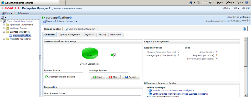
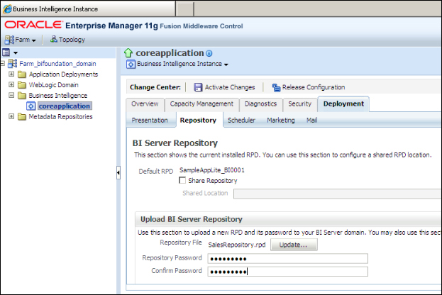
When you log in, you'll see the Deployment tab and the Repository link. This is the page that we're going to upload the repository to. You'll have to show the path of the existing repository and specify the password in Repository Password.
Restart the service in order to use the new repository. Now we can run tests, but it's better to increase the logging level and also see the queries that are executed on the physical data sources. When you open BI Administration Tool in online mode, you'll be able to download the user information from the WebLogic Server and change the logging level.
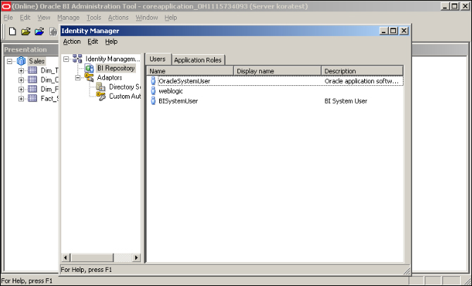
Open the properties of the user account that you'll run tests on. In our scenario, we're going to use
weblogicuser account and change the value in Logging level to2. This level is going to force the BI server to generate both the logical as well as the physical SQL statements.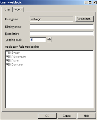
Now we can run our tests easily. We're going to use the web browser to access Presentation Service at
http://localhost:7001/analytics.
After you log in and try to create an analysis, you'll see the subject area from the Presentation layer of the repository. Click on the Subject Area name.

It's going to open the Analysis Editor. You'll see that the order of the tables and columns are exactly the same as the order of the subject areas in the Presentation layer. You can easily click on the columns from the Subject Areas pane to add them to the Selected Columns section.
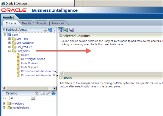
Click on the Results tab on this page to see the results:

After uploading the new repository to the BI server, we'll have to make many tests in order to make sure that everything is fine. Also, logs should be checked.
To make a test, we'll have to log in to Presentation Services and create analysis. After clicking the Results tab, we should see the result set as shown in the preceding example. The logical request is going to be constructed from the definition of the analysis at the Presentation Services and it'll be retrieved by the BI server component. The BI server is going to convert the logical SQL statement to a physical SQL statement and execute it against the database. After the result set is generated by the database, that result set is going to pass through the BI server and will be listed as a result at the Presentation Services.
After changing the log level of the user that we're running the test on, we can find the execution statistics in the log file. The name of the log file is NQQuery.log. The content of the log file can be accessed from the Administration link in Presentation Services by navigating to Administration | Manage Sessions | View Log.