


In this chapter, we will cover the following recipes:
Installing IPython
Using IPython as a shell
Reading manual pages
Installing matplotlib
Running an IPython notebook
Exporting an IPython notebook
Importing a web notebook
Configuring a notebook server
Exploring the SymPy profile
IPython, which is available at http://ipython.org/, is a free, open source project available for Linux, Unix, Mac OS X, and Windows. The IPython authors only request that you cite IPython in any scientific work where IPython was used. IPython provides an architecture for interactive computing. The most notable part of this project is the IPython shell. IPython provides the following components, among others:
Interactive Python shells (terminal-based and Qt application)
A web notebook (available in IPython 0.12 and later) with support for rich media and plotting
IPython is compatible with Python versions 2.5, 2.6, 2.7, 3.1, 3.2, 3.3, and 3.4. The compatibility depends on the IPython version. For instance, IPython 2.3.0 requires Python 2.7 or 3.3+.
You can try IPython in the cloud without installing it on your system by going to http://www.pythonanywhere.com/try-ipython/. There is a slight delay compared to locally installed software, so this is not as good as the real thing. However, most of the features available in the IPython interactive shell seem to be available. PythonAnywhere also has a Vi (m) editor, which if you like vi, is obviously great. You can save and edit files from your IPython sessions.
IPython can be installed in various ways, depending on your operating system. For the terminal-based shell, there is a dependency on readline. The web notebook requires tornado and zmq.
In addition to installing IPython, we will install setuptools, which gives you the easy_install command. The easy_install command is a popular package manager for Python. pip can be installed once you have easy_install. The pip command is similar to easy_install and adds options such as uninstalling.
This section describes how IPython can be installed on Windows, Mac OS X, and Linux. It also describes how to install IPython and its dependencies with easy_install and pip, or from source:
Installing IPython and setuptools on Windows: A binary Windows installer for Python 2 or Python 3 is available on the IPython website. Also see http://ipython.org/ipython-doc/stable/install/install.html#windows.
Install setuptools with an installer from http://pypi.python.org/pypi/setuptools#files. Then install
pip, like this:cd C:\Python27\scripts python .\easy_install-27-script.py pip
Installing IPython on Mac OS X: Install the Apple Developer Tools (Xcode) if necessary. Xcode can be found at https://developer.apple.com/xcode/. Follow the
easy_install/pipinstructions or the instructions for installation from source provided later in this section.Installing IPython on Linux: Since there are so many Linux distributions, this section will not be exhaustive:
On Debian, type the following command:
$ su – aptitude install ipython python-setuptoolsOn Fedora, the magic command is as follows:
$ su – yum install ipython python-setuptools-develThe following command will install IPython on Gentoo:
$ su – emerge ipythonFor Ubuntu, the install command is as follows:
$ sudo apt-get install ipython python-setuptools
Installing IPython with easy_install or pip: Install IPython and all the dependencies required for the recipes in this chapter with
easy_installusing the following command:$ sudo easy_install ipython pyzmq tornado readlineAlternatively, you can first install pip with
easy_installby typing this command in your terminal:$ sudo easy_install pipAfter that, install IPython using
pip:$ sudo pip install ipython pyzmq tornado readlineInstalling from source: If you want to use the bleeding-edge development version, then installing from source is for you:
Download the latest source archive from https://github.com/ipython/ipython/archive/master.zip.
Unpack the source code from the archive:
$ tar xzf ipython-<version>.tar.gzInstead, if you have Git installed, you can clone the Git repository:
$ git clone https://github.com/ipython/ipython.gitGo to the root directory within the downloaded source:
$ cd ipythonRun the setup script. This may require you to run the command with
sudo, as follows:$ sudo python setup.py install
We installed IPython using several methods. Most of these methods install the latest stable release, except when you install from source, which will install the development version.
Instructions from the official IPython website at http://ipython.org/install.html
Scientists and engineers are used to experimenting. IPython was created by scientists with experimentation in mind. The interactive environment that IPython provides is viewed by many as a direct answer to MATLAB, Mathematica, Maple, and R.
The following is a list of features of the IPython shell:
Tab completion
History mechanism
Inline editing
The ability to call external Python scripts with
%runThe ability to call magic functions that interact with the operating system shell
Access to system commands
The
pylabswitchAccess to Python debugger and profiler
This section describes how to use the IPython shell:
pylab: Thepylabswitch automatically imports all the SciPy, NumPy, and matplotlib packages. Without this switch, we would have to import these packages ourselves.All we need to do is enter the following instruction on the command line:
$ ipython --pylab
Type "copyright", "credits" or "license" for more information.

IPython 2.4.1 -- An enhanced Interactive Python.
?         -> Introduction and overview of IPython's features.
%quickref -> Quick reference.
help      -> Python's own help system.
object?   -> Details about 'object', use 'object??' for extra details.

Welcome to pylab, a matplotlib-based Python environment [backend: MacOSX].
For more information, type 'help(pylab)'.

In [1]: quit()
quit() or Ctrl + D quits the IPython shell.
Saving a session: We might want to be able to go back to our experiments. In IPython, it is easy to save a session for later use. This is done with the following command:
In [1]: %logstart
Activating auto-logging. Current session state plus future input saved.
Filename       : ipython_log.py
Mode           : rotate
Output logging : False
Raw input log  : False
Timestamping   : False
State          : active
Logging can be switched off using this command:
In [9]: %logoff
Switching logging OFF
Executing a system shell command: You can execute a system shell command in the default IPython profile by prefixing the command with the
!symbol. For instance, the following input will get the current date:In [1]: !dateIn fact, any line prefixed with
!is sent to the system shell. We can also store the command output, as shown here:In [2]: thedate = !date In [3]: thedate
Displaying history: We can show the history of commands with the
%histcommand, like this:In [1]: a = 2 + 2 In [2]: a Out[2]: 4 In [3]: %hist a = 2 + 2 a %hist
This is a common feature in Command-line Interface (CLI) environments. We can also look up the history with the
-gswitch:In [5]: %hist -g a = 2 1: a = 2 + 2
Tip
Downloading the example code
You can download the example code files for all Packt Publishing books you have purchased from your account at http://www.packtpub.com. If you purchased this book elsewhere, you can visit http://www.packtpub.com/support and register to get the files e-mailed directly to you.
We saw a number of so-called magic functions in action. These functions start with the % character. If a magic function is used in a line by itself, the % prefix is optional.
IPython as a system shell from the official IPython website at http://ipython.org/ipython-doc/dev/interactive/shell.html
We can open the documentation for NumPy functions with the help command. It is not necessary to know the name of a function. We can type a few characters and then let tab completion do its work. For instance, let's browse the available information for the arange() function.
We can browse the available information in either of the following ways:
Calling the help function: Call the
helpcommand. Type a few characters of the function and then press the Tab key (see the following screenshot):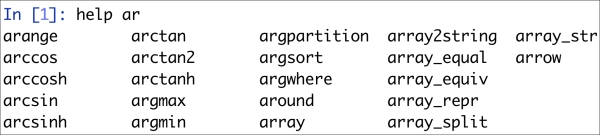
Querying with a question mark: Another option is to put a question mark behind the function name. You will then, of course, need to know the function name, but you don't have to type the
helpcommand:In [3]: arange?
matplotlib (all lowercase by convention) is a very useful Python plotting library, and we will need it for the following recipes as well as more later on. It depends on NumPy, but in all likelihood, you already have NumPy installed.
We will see how matplotlib can be installed on Windows, Linux, and Mac OS X, and also how to install it from source:
Installing matplotlib on Windows: You can install this with the Enthought distribution, also known as Canopy (http://www.enthought.com/products/epd.php).
It might be necessary to put the
msvcp71.dllfile in yourC:\Windows\system32directory. You can get it from http://www.dll-files.com/dllindex/dll-files.shtml?msvcp71.Installing matplotlib on Linux: Let's see how matplotlib can be installed in the various distributions of Linux:
Here is the install command on Debian and Ubuntu:
$ sudo apt-get install python-matplotlibThe install command on Fedora/Redhat is as follows:
$ su - yum install python-matplotlib
Installing from source: You can download the latest source from the
tar.gzrelease at Sourceforge (http://sourceforge.net/projects/matplotlib/files/), or from the Git repository using the following command:$ git clone git://github.com/matplotlib/matplotlib.gitOnce it has been downloaded, build and install matplotlib as usual with the following commands:
$ cd matplotlib
$ sudo python setup.py install
Installing matplotlib on Mac OS X: Get the latest DMG file from http://sourceforge.net/projects/matplotlib/files/matplotlib/ and install it. You can also use the Mac Ports, Fink, or Homebrew package managers.
Instructions from the official matplotlib documentation are given at http://matplotlib.org/users/installing.html
Installing the SciPy stack is explained at http://www.scipy.org/install.html
IPython has an exciting feature—the web notebook. A so-called notebook server can serve notebooks over the Web. We can now start a notebook server and get a web-based IPython environment. This environment has most of the features that the regular IPython environment has. The IPython notebook's features include the following:
Displaying images and inline plots
Using HTML and Markdown (this is a simplified HTML-like language see https://en.wikipedia.org/wiki/Markdown) in text cells
Importing and exporting of notebooks
Before we start, we should make sure that all of the required software is installed. There is a dependency on tornado and zmq. See the Installing IPython recipe in this chapter for more information.
Running a notebook: We can start a notebook with the following command:
$ ipython notebook

[NotebookApp] Using existing profile dir: u'/Users/ivanidris/.ipython/profile_default'
[NotebookApp] The IPython Notebook is running at: http://127.0.0.1:8888
[NotebookApp] Use Control-C to stop this server and shut down all kernels.
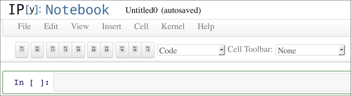
As you can see, we are using the default profile. A server started on the local machine at port 8888. You will learn how to configure these settings later on in this chapter. The notebook is opened in your default browser; this is configurable as well (see the following screenshot):

IPython lists all the notebooks in the directory where you started the notebook. In this example, no notebooks were found. The server can be stopped by pressing Ctrl + C.
Running a notebook in the pylab mode: Run a web notebook in the pylab mode with the following command:
$ ipython notebook --pylabThis loads the
SciPy,NumPy, andmatplotlibmodules.Running a notebook with inline figures: We can display inline matplotlib plots with the
inlinedirective using the following command:$ ipython notebook --pylab inlineThe following steps demonstrate the IPython notebook functionality:
Click on the New Notebook button to create a new notebook.
Create an array with the
arange()function. Type the command shown in the following screenshot and click on Cell/Run:
Next enter the following command and press Enter. You will see the output in Out [2], as shown in the following screenshot:

Apply the
sinc()function to the array and plot the result, as shown in this screenshot:

The inline option lets you display inline matplotlib plots. When combined with the pylab mode, you don't need to import the NumPy, SciPy, and matplotlib packages.
The Installing IPython recipe found in this chapter
Example notebooks at http://nbviewer.ipython.org/github/ipython/ipython/blob/2.x/examples/Notebook/Index.ipynb
Documentation for the
sinc()function at http://docs.scipy.org/doc/numpy/reference/generated/numpy.sinc.htmlDocumentation for the
plot()function at http://matplotlib.org/api/pyplot_api.html#matplotlib.pyplot.plot
Sometimes, you would want to exchange notebooks with friends or colleagues. The web notebook provides several methods to export your data.
A web notebook can be exported using the following options:
The Print option: The Print button doesn't actually print the notebook, but allows you to export the notebook as a PDF or HTML document.
Downloading the notebook: Download your notebook to a location chosen by you, using the Download button. We can specify whether we want to download the notebook as a
.pyfile, which is just a normal Python program, or in the JSON format as a.ipynbfile. The notebook we created in the previous recipe looks like the following after exporting:{ "metadata": { "name": "Untitled1" }, "nbformat": 2, "worksheets": [ { "cells": [ { "cell_type": "code", "collapsed": false, "input": [ "plot(sinc(a))" ], "language": "python", "outputs": [ { "output_type": "pyout", "prompt_number": 3, "text": [ "[<matplotlib.lines.Line2D at 0x103d9c690>]" ] }, { "output_type": "display_data", "png": "iVBORw0KGgoAAAANSUhEUgAAAXkAAAD9CAYAAABZVQdHAAAABHNCSVQICAgIf... mgkAAAAASUVORK5CYII=\n" } ], "prompt_number": 3 } ] } ] }Note
Some of the text has been omitted for brevity. This file is not intended for editing or even reading, but it is pretty readable if you ignore the image representation part. For more information about JSON, see https://en.wikipedia.org/wiki/JSON.

A public notebook server needs to be secure. You should set a password and use an SSL certificate to connect to it. We need the certificate to provide secure communication over HTTPS (for more information, see https://en.wikipedia.org/wiki/Transport_Layer_Security). HTTPS adds a secure layer on top of the standard HTTP protocol widely used on the Internet. HTTPS also encrypts data sent from the client to the server and back. A certificate authority is often a commercial organization that issues certificates for websites. Web browsers have knowledge of certificate authorities and can recognize certificates. A website administrator needs to create a certificate and get it signed by a certificate authority.
The following steps describe how to configure a secure notebook server:
We can generate a password from IPython. Start a new IPython session and type in the following commands:
In [1]: from IPython.lib import passwd

In [2]: passwd()
Enter password:
Verify password:
Out[2]: 'sha1:0e422dfccef2:84cfbcbb3ef95872fb8e23be3999c123f862d856'
At the second input line, you will be prompted for a password. You need to remember this password. A long string is generated. Copy this string because you will need it later on.
To create a SSL certificate, you will need the
opensslcommand in your path.Setting up the
opensslcommand is not rocket science, but it can be tricky. Unfortunately, it is outside the scope of this book. On the brighter side, there are plenty of tutorials available online to help you further.Execute the following command to create a certificate with
mycert.pemas the name:$ openssl req -x509 -nodes -days 365 -newkey rsa:1024 -keyout mycert.pem -out mycert.pem Generating a 1024 bit RSA private key ......++++++ ........................++++++ writing new private key to 'mycert.pem' ----- You are about to be asked to enter information that will be incorporated into your certificate request. What you are about to enter is what is called a Distinguished Name or a DN. There are quite a few fields but you can leave some blank For some fields there will be a default value, If you enter '.', the field will be left blank. ----- Country Name (2 letter code) [AU]: State or Province Name (full name) [Some-State]: Locality Name (eg, city) []: Organization Name (eg, company) [Internet Widgits Pty Ltd]: Organizational Unit Name (eg, section) []: Common Name (eg, YOUR name) []: Email Address []:
The
opensslutility prompts you to fill in some fields. For more information, check out the relevant man page (short for manual page) as follows:$ man opensslCreate a special profile for the server using the following command:
$ ipython profile create nbserverEdit the configuration file. In this example, it can be found in
~/.ipython/profile_nbserver/ipython_notebook_config.py.The configuration file is pretty large, so we will omit most of the lines in it. The lines that we need to change at minimum are as follows:
c.NotebookApp.certfile = u'/absolute/path/to/your/certificate'
c.NotebookApp.password = u'sha1:b...your password'
c.NotebookApp.port = 9999
Notice that we are pointing to the SSL certificate we created. We set a password and changed the port to 9999.
Using the following command, start the server to check whether the changes worked:
$ ipython notebook --profile=nbserver
[NotebookApp] Using existing profile dir: u'/Users/ivanidris/.ipython/profile_nbserver'
[NotebookApp] The IPython Notebook is running at: https://127.0.0.1:9999
[NotebookApp] Use Control-C to stop this server and shut down all kernels.
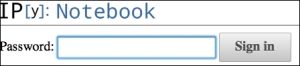
The server is running on port 9999, and you need to connect to it via https. If everything goes well, you should see a login page. Also, you will probably need to accept a security exception in your browser.
We created a special profile for our public server. There are some sample profiles that are already present, such as the default profile. Creating a profile adds a profile_<profilename> folder to the .ipython directory with a configuration file, among others. The profile can then be loaded with the --profile=<profile_name> command-line option. We can list the profiles with the following command:
$ ipython profile list

Available profiles in IPython:
    cluster
    math
    pysh
    python3

    The first request for a bundled profile will copy it
    into your IPython directory (/Users/ivanidris/.ipython),
    where you can customize it.

Available profiles in /Users/ivanidris/.ipython:
    default
    nbserver
    sh
IPython documentation for the
passwd()function at http://ipython.org/ipython-doc/2/api/generated/IPython.lib.security.htmlOpenSSL documentation at https://www.openssl.org/docs/apps/openssl.html
IPython has a sample SymPy profile. SymPy is a Python-symbolic mathematics library. We can simplify algebraic expressions or differentiate functions, similar to Mathematica and Maple. SymPy is obviously a fun piece of software, but is not necessary for our journey through the NumPy landscape. Consider this as an optional or bonus recipe. Like a dessert, feel free to skip it, although you might miss out on the sweetest piece of this chapter.
Install SymPy using either easy_install or pip:
$ sudo easy_install sympy
$ sudo pip install sympy
The following steps will help you explore the SymPy profile:
Look at the configuration file, which can be found at
~/.ipython/profile_sympy/ipython_config.py. The content is as follows:c = get_config() app = c.InteractiveShellApp # This can be used at any point in a config file to load a sub config # and merge it into the current one. load_subconfig('ipython_config.py', profile='default') lines = """ from __future__ import division from sympy import * x, y, z, t = symbols('x y z t') k, m, n = symbols('k m n', integer=True) f, g, h = symbols('f g h', cls=Function) """ # You have to make sure that attributes that are containers already # exist before using them. Simple assigning a new list will override # all previous values. if hasattr(app, 'exec_lines'): app.exec_lines.append(lines) else: app.exec_lines = [lines] # Load the sympy_printing extension to enable nice printing of sympy expr's. if hasattr(app, 'extensions'): app.extensions.append('sympyprinting') else: app.extensions = ['sympyprinting']
This code accomplishes the following:
Loads the default profile
Imports the SymPy packages
Defines symbols
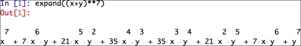
Start IPython with the SymPy profile using this command:
$ ipython --profile=sympyExpand an algebraic expression using the command shown in the following screenshot:
The SymPy homepage at http://sympy.org/en/index.html

