


Let's get started. We will install NumPy on different operating systems and have a look at some simple code that uses NumPy. The IPython interactive shell is introduced briefly. As mentioned in the preface, SciPy is closely related to NumPy, so you will see the SciPy name appearing here and there. At the end of this chapter, you will find pointers on how to find additional information online if you get stuck or are uncertain about the best way to solve problems.
In this chapter, we shall:
Install Python and NumPy on Windows
Install Python and NumPy on Linux
Install Python and NumPy on Macintosh
Write simple NumPy code
Get to know IPython
Browse online documentation and resources
NumPy has binary installers for Windows, various Linux distributions and Mac OS X. There is also a source distribution, if you prefer that. You need to have Python 2.4.x or above installed on your system. We will go through the various steps required to install Python on the following operating systems:
Debian and Ubuntu : Python might already be installed on Debian and Ubuntu but the development headers are usually not. On Debian and Ubuntu install python and python-dev with the following commands:
sudo apt-get install python
sudo apt-get install python-dev
Windows : The Windows Python installer can be found at www.python.org/download. On this website, we can also find installers for Mac OS X and source tarballs for Linux, Unix, and Mac OS X.
Mac: Python comes pre-installed on Mac OS X . We can also get Python through MacPorts, Fink, or similar projects.
We can install, for instance, the Python 2.6 port by running the following command:
sudo port install python26
LAPACKdoes not need to be present but, if it is, NumPy will detect it and use it during the installation phase. It is recommended to installLAPACKfor serious numerical analysis.
We installed Python on Debian, Ubuntu, Windows, and the Mac.
Tip
Downloading the example code
You can download the example code files for all Packt books you have purchased from your account at http://www.PacktPub.com. If you purchased this book elsewhere, you can visit http://www.PacktPub.com/support and register to have the files e-mailed directly to you.
Installing NumPy on Windows is necessary but, fortunately, a straightforward task. The actions we will take are as follows:
Download the NumPy installer: Download a NumPy installer for Windows from the SourceForge website http://sourceforge.net/projects/numpy/files/
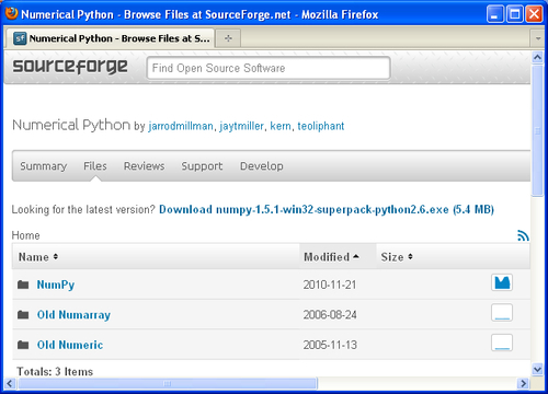
Choose the appropriate version. In this example, we chose
numpy-1.5.1-win32-superpack-python2.6.exe.Open the installer: Open the EXE installer by double clicking on it.
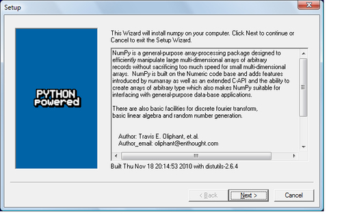
NumPy features: Now, we see a description of NumPy and its features. Click Next.
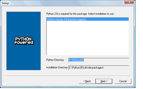
Install Python: If you have Python installed, it should automatically be detected. If it is not detected, maybe your path settings are wrong. At the end of this chapter, resources are listed in case you have problems with installing NumPy:
Finish the installation: In this example, Python 2.6 was found. Click Next if Python is found; otherwise, click Cancel and install Python (NumPy cannot be installed without Python). Click Next. This is the point of no return. Well, kind of, but it is best to make sure that you are installing to the proper directory and so on and so forth. Now the real installation starts. This may take a while:
Most Linux distributions have NumPy packages. We will go through the necessary steps for some of the popular Linux distros:
Installing NumPy on Red Hat: Run the following instructions from the command line:
yum install python-numpy
Installing NumPy on Mandriva : To install NumPy on Mandriva, run the following command line instruction:
urpmi python-numpy
Installing NumPyon Gentoo : To install NumPy on Gentoo run the following command line instruction:
sudo emerge numpy
Installing NumPyon Debian andUbuntu : On Debian or Ubuntu, we need to type the following:
sudo apt-get install python-numpy
The following table gives an overview of the Linux distributions and corresponding NumPy package names.
|
python-numpy | |
We will install NumPy with a GUI installer.
Download the GUI installer: We can get a NumPy installer from the SourceForge website http://sourceforge.net/projects/numpy/files/. Download the appropriate
DMGfile. Usually the latest one is the best: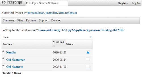
Open the DMG file : Open the DMG file (in this example,
numpy-1.5.1-py2.6-python.org-macosx10.3.dmg):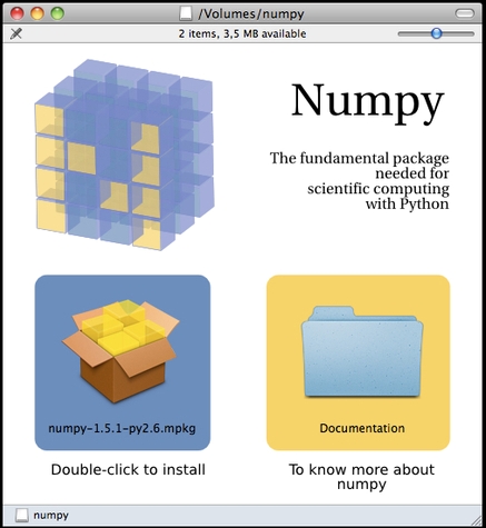
Double-click on the icon of the opened box, the one having a subscript that ends with .mpkg. We will be presented with the welcome screen of the installer.
Click on the Continue button to go to the ReadMe screen, where we will be presented with a short description of NumPy:
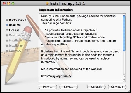
Continue to the License screen.
Accept the license: Read the license, click Continue and then the Accept button, when prompted to accept the license. Continue through the next screens and click Finish at the end.
We can retrieve the source code for NumPy with
git. This is shown as follows:
git clone git://github.com/numpy/numpy.git numpy
Install /usr/local with the following command:
python setup.py buildsudo python setup.py install --prefix=/usr/local
To build, we need a C compiler such as GCC and the Python header files in the python-dev or python-devel package.
Imagine that we want to add two vectors called a and b. Vector a holds the squares of integers 0 to n, for instance, if n = 3, then a = (0, 1, 4). Vector b holds the cubes of integers 0 to n, so if n = 3, then b = (0, 1, 8). How would you do that using plain Python? After we come up with a solution, we will compare it with the NumPy equivalent.
Adding vectors using pure Python: The following function solves the vector addition problem using pure Python without NumPy:
def pythonsum(n):
   a = range(n)
   b = range(n)
   c = []

   for i in range(len(a)):
       a[i] = i ** 2
       b[i] = i ** 3
       c.append(a[i] + b[i])

   return c
Adding vector susing NumPy: Following is a function that achieves the same with NumPy.
def numpysum(n):
  a = numpy.arange(n) ** 2
  b = numpy.arange(n) ** 3
  c = a + b
  return c
Notice that numpysum() does not need a for loop. Also, we used the arange function from NumPy that creates a NumPy array for us with integers 0 to n. The arange function was imported; that is why it is prefixed with numpy.
Now comes the fun part. Remember that it is mentioned in the preface that NumPy is faster when it comes to array operations. How much faster is Numpy, though? The following program will show us by measuring the elapsed time in microseconds, for the numpysum
and
pythonsum functions. It also prints the last two elements of the vector sum. Let's check that we get the same answers by using Python and NumPy:
import sys
from datetime import datetime
import numpy

def numpysum(n):
  a = numpy.arange(n) ** 2
  b = numpy.arange(n) ** 3
  c = a + b
  return c

def pythonsum(n):
   a = range(n)
   b = range(n)
   c = []

   for i in range(len(a)):
       a[i] = i ** 2
       b[i] = i ** 3
       c.append(a[i] + b[i])

   return c

size = int(sys.argv[1])
start = datetime.now()
c = pythonsum(size)
delta = datetime.now() - start
print "The last 2 elements of the sum", c[-2:]
print "PythonSum elapsed time in microseconds", delta.microseconds
start = datetime.now()
c = numpysum(size)
delta = datetime.now() - start
print "The last 2 elements of the sum", c[-2:]
print "NumPySum elapsed time in microseconds", delta.microseconds
The output of the program for 1000, 2000, and 3000 vector elements is as follows:
$ python vectorsum.py 1000The last 2 elements of the sum [995007996, 998001000]PythonSum elapsed time in microseconds 707The last 2 elements of the sum [995007996 998001000]NumPySum elapsed time in microseconds 171
$ python vectorsum.py 2000The last 2 elements of the sum [7980015996, 7992002000]PythonSum elapsed time in microseconds 1420The last 2 elements of the sum [7980015996 7992002000]NumPySum elapsed time in microseconds 168
$ python vectorsum.py 4000The last 2 elements of the sum [63920031996, 63968004000]PythonSum elapsed time in microseconds 2829The last 2 elements of the sum [63920031996 63968004000]NumPySum elapsed time in microseconds 274
Clearly, NumPy is much faster than the equivalent normal Python code. One thing is certain; we get the same results whether we are using NumPy or not. However, the result that is printed differs in representation. Notice that the result from the numpysum function does not have any commas. How come? Obviously we are not dealing with a Python list but with a NumPy array. It was mentioned in the preface that NumPy arrays are specialized data structures for numerical data. We will learn more about NumPy arrays in the next chapter.
What does
arange(5)do?Creates a Python list of 5 elements with values 1 to 5.
Creates a Python list of 5 elements with values 0 to 4.
Creates a NumPy array with values 1 to 5.
Creates a NumPy array with values 0 to 4.
None of the above.
The program we used here to compare the speed of NumPy and regular Python is not very scientific. We should at least repeat each measurement a couple of times. It would be nice to be able to calculate some statistics such as average times, and so on. Also, you might want to show plots of the measurements to friends and colleagues.
Scientists and engineers are used to experimenting. IPython was created by scientists with experimentation in mind. The interactive environment that IPython provides is viewed by many as a direct answer to Matlab, Mathematica, and Maple. You can find more information, including installation instructions, at: http://ipython.org/
IPython is free, open source, and available for Linux, Unix, Mac OS X, and Windows. The IPython authors only request that you cite IPython in scientific work where IPython was used. Here is the list of features of IPython:
The Pylab switch imports all the Scipy, NumPy, and Matplotlib packages. Without this switch, we would have to import every package we need ourselves.
All we need to do is enter the following instruction on the command line:
$ ipython -pylab
Python 2.6.1 (r261:67515, Jun 24 2010, 21:47:49)
Type "copyright", "credits" or "license" for more information.

IPython 0.10 -- An enhanced Interactive Python.
?         -> Introduction and overview of IPython's features.
%quickref -> Quick reference.
help      -> Python's own help system.
object?   -> Details about 'object'. ?object also works, ?? prints more.

  Welcome to pylab, a matplotlib-based Python environment.
  For more information, type 'help(pylab)'.

In [1]: quit()
quit()
or Ctrl + D quits the IPython shell. We might want to be able to go back to our experiments. In IPython, it is easy to save a session for later.
In [1]: %logstart
Activating auto-logging. Current session state plus future input saved.
Filename       : ipython_log.py
Mode           : rotate
Output logging : False
Raw input log  : False
Timestamping   : False
State          : active
Let's say we have the vector addition program that we made in the current directory. We can run the script as follows:
In [1]: ls
README        vectorsum.py

In [2]: %run -i vectorsum.py 1000
As you probably remember, 1000 specifies the number of elements in a vector. The -d switch of %run starts an ipdb debugger with 'c' the script is started. 'n' steps through the code. Typing quit at the ipdb prompt exits the debugger.
In [2]: %run -d vectorsum.py 1000
*** Blank or comment
*** Blank or comment
Breakpoint 1 at /Users/ivanidris/Documents/numpyBeginnersGuide/book/ch1code/vectorsum.py:3
><string>(1)<module>()

ipdb> c
> /Users/ivanidris/Documents/numpyBeginnersGuide/book/ch1code/vectorsum.py(3)<module>()
      2
1---> 3 import sys
      4 from datetime import datetime

ipdb> n
> /Users/ivanidris/Documents/numpyBeginnersGuide/book/ch1code/vectorsum.py(4)<module>()
1     3 import sys
----> 4 from datetime import datetime
      5 import numpy

ipdb> n
> /Users/ivanidris/Documents/numpyBeginnersGuide/book/ch1code/vectorsum.py(5)<module>()
      4 from datetime import datetime
----> 5 import numpy
      6

ipdb> quit
We can also profile our script by passing the -p option to %run.
In [4]: %run -p vectorsum.py 1000
         1058 function calls (1054 primitive calls) in 0.002 CPU seconds

   Ordered by: internal time

ncallstottimepercallcumtimepercallfilename:lineno(function)
        1    0.001    0.0010.0010.001 vectorsum.py:28(pythonsum)
        1    0.001    0.001    0.002    0.002 {execfile}
     1000    0.000    0.0000.0000.000 {method 'append' of 'list' objects}
        1    0.000    0.000    0.002    0.002 vectorsum.py:3(<module>)
        1    0.000    0.0000.0000.000 vectorsum.py:21(numpysum)
        3    0.000    0.0000.0000.000 {range}
        1    0.000    0.0000.0000.000 arrayprint.py:175(_array2string)
      3/1    0.000    0.0000.0000.000 arrayprint.py:246(array2string)
        2    0.000    0.0000.0000.000 {method 'reduce' of 'numpy.ufunc' objects}
        4    0.000    0.0000.0000.000 {built-in method now}
        2    0.000    0.0000.0000.000 arrayprint.py:486(_formatInteger)
        2    0.000    0.0000.0000.000 {numpy.core.multiarray.arange}
        1    0.000    0.0000.0000.000 arrayprint.py:320(_formatArray)
      3/1    0.000    0.0000.0000.000 numeric.py:1390(array_str)
        1    0.000    0.0000.0000.000 numeric.py:216(asarray)
        2    0.000    0.0000.0000.000 arrayprint.py:312(_extendLine)
        1    0.000    0.0000.0000.000 fromnumeric.py:1043(ravel)
        2    0.000    0.0000.0000.000 arrayprint.py:208(<lambda>)
        1    0.000    0.000    0.002    0.002<string>:1(<module>)
       11    0.000    0.0000.0000.000 {len}
        2    0.000    0.0000.0000.000 {isinstance}
        1    0.000    0.0000.0000.000 {reduce}
        1    0.000    0.0000.0000.000 {method 'ravel' of 'numpy.ndarray' objects}
        4    0.000    0.0000.0000.000 {method 'rstrip' of 'str' objects}
        3    0.000    0.0000.0000.000 {issubclass}
        2    0.000    0.0000.0000.000 {method 'item' of 'numpy.ndarray' objects}
        1    0.000    0.0000.0000.000 {max}
        1    0.000    0.0000.0000.000 {method 'disable' of '_lsprof.Profiler' objects}
This gives us a bit more insight in the workings of our program. In addition, we can now identify performance bottlenecks. The %hist command shows the commands history.
In [2]: a=2+2

In [3]: a
Out[3]: 4

In [4]: %hist
1: _ip.magic("hist ")
2: a=2+2
3: a
I hope you agree that IPython is a really useful tool!
When we are in IPython's pylab mode, we can open manual pages for NumPy functions with the help command. It is not necessary to know the name of a function. We can type a few characters and then let tab completion do its work. Let's, for instance, browse the available information for the arange function.
In [2]: help ar<Tab>
arangearccosarccosharcsinarcsinh
arctan        arctan2       arctanhargmaxargmin
argsortargwhere      around        array2string  array_equal
array_equivarray_reprarray_splitarray_str     arrow
array

In [2]: help arange
Another option is to put a question mark behind the function name.
In [3]: arange?
The main documentation website for NumPy and SciPy is at http://docs.scipy.org/doc/. Through this webpage, we can browse the NumPy reference at http://docs.scipy.org/doc/numpy/reference/ and the user guide as well as several tutorials.
NumPy has a wiki with lots of documentation at http://docs.scipy.org/numpy/Front%20Page/.
The NumPy and SciPy forum can be found at http://ask.scipy.org/en.
The popular Stack Overflow software development forum has hundreds of questions tagged "numpy". To view them, go to http://stackoverflow.com/questions/tagged/numpy.
If you are really stuck with a problem or you want to be kept informed of NumPy development, you can subscribe to the NumPy discussion mailing list. The e-mail address is <numpy-discussion@scipy.org>. The number of e-mails per day is not too high and there is almost no spam to speak of. Most importantly, developers actively involved with NumPy also answer questions asked on the discussion group. The complete list can be found at http://www.scipy.org/Mailing_Lists.
For IRC users, there is an IRC channel on irc.freenode.net. The channel is called #scipy
, but you can also ask NumPy questions since SciPy users also have knowledge of NumPy, as SciPy is based on NumPy. There are at least 50 members on the scipy channel at all times.
In this chapter, we installed NumPy. We got a vector addition program working and convinced ourselves that NumPy has superior performance. We were introduced to the IPython interactive shell. In addition, we explored the available NumPy documentation and online resources.
In the next chapter, we will take a look under the hood and explore some fundamental concepts including arrays and data types.
