Neural Network Programming with Tensorflow

Before we jump into the field of mathematics and its properties, it's essential for us to set up the development environment as it will provide us settings to execute the concepts we learn, meaning installing the compiler, dependencies, and IDE (Integrated Development Environment) to run our code base.

Setting up the Python environment in Pycharm

It is best to use an IDE like Pycharm to edit Python code as it provides development tools and built-in coding assistance. Code inspection makes coding and debugging faster and simpler, ensuring that you focus on the end goal of learning maths for neural networks.

The following steps show you how to set up local Python environment in Pycharm:

1. Go to Preferences and verify that the TensorFlow library is installed. If not, follow the instructions at https://www.tensorflow.org/install/ to install TensorFlow:

2. Keep the default options of TensorFlow and click on OK.
3. Finally, right-click on the source file and click on Run 'matrices':

In the following section, we will describe the fundamental structures of linear algebra.

Tensors

An array of numbers with a variable number of axes is known as a tensor. For example, for three axes, it is identified using three indices (i, j, k). 

The following image summaries a tensor, it describes a second-order tensor object. In a three-dimensional Cartesian coordinate system, tensor components will form the matrix:

      

Note

Image reference is taken from tensor wiki https://en.wikipedia.org/wiki/Tensor

The following topics will describe the various operations of linear algebra.

Vectors

The Normfunction is used to get the size of the vector; the norm of a vector x measures the distance from the origin to the point x. It is also known as the

norm, where p=2 is known as the Euclidean norm.

The following example shows you how to calculate the

norm of a given vector:

import tensorflow as tf

vector = tf.constant([[4,5,6]], dtype=tf.float32)
eucNorm = tf.norm(vector, ord="euclidean")

with tf.Session() as sess:
print(sess.run(eucNorm))

The output of the listing is 8.77496.

# convert matrices to tensor objects
import numpy as np
import tensorflow as tf

# create a 2x2 matrix in various forms
matrix1 = [[1.0, 2.0], [3.0, 40]]
matrix2 = np.array([[1.0, 2.0], [3.0, 40]], dtype=np.float32)
matrix3 = tf.constant([[1.0, 2.0], [3.0, 40]])

print(type(matrix1))
print(type(matrix2))
print(type(matrix3))

tensorForM1 = tf.convert_to_tensor(matrix1, dtype=tf.float32)
tensorForM2 = tf.convert_to_tensor(matrix2, dtype=tf.float32)
tensorForM3 = tf.convert_to_tensor(matrix3, dtype=tf.float32)

print(type(tensorForM1))
print(type(tensorForM2))
print(type(tensorForM3))

<class 'list'>
<class 'numpy.ndarray'>
<class 'tensorflow.python.framework.ops.Tensor'>
<class 'tensorflow.python.framework.ops.Tensor'>
<class 'tensorflow.python.framework.ops.Tensor'>
<class 'tensorflow.python.framework.ops.Tensor'>

Matrix multiplication

Matrix multiplication of matrices A and B is a third matrix, C:

C = AB

The element-wise product of matrices is called a Hadamard product and is denoted as A.B.

The dot product of two vectors x and y of the same dimensionality is the matrix product x transposing y. Matrix product C = AB is like computing C_i,j as the dot product between row i of matrix A and column j of matrix B:

The following example shows the Hadamard product and dot product using tensor objects:

import tensorflow as tf

mat1 = tf.constant([[4, 5, 6],[3,2,1]])
mat2 = tf.constant([[7, 8, 9],[10, 11, 12]])

# hadamard product (element wise)
mult = tf.multiply(mat1, mat2)

# dot product (no. of rows = no. of columns)
dotprod = tf.matmul(mat1, tf.transpose(mat2))

with tf.Session() as sess:
    print(sess.run(mult))
    print(sess.run(dotprod))

The output of the listing is shown as follows:

[[28 40 54][30 22 12]]
 [[122 167][ 46 64]]

import tensorflow as tf

mat = tf.constant([
 [0, 1, 2],
 [3, 4, 5],
 [6, 7, 8]
], dtype=tf.float32)

# get trace ('sum of diagonal elements') of the matrix
mat = tf.trace(mat)

with tf.Session() as sess:
    print(sess.run(mat))

Matrix transpose

Transposition of the matrix is the mirror image of the matrix across the main diagonal. A symmetric matrix is any matrix that is equal to its own transpose:

The following example shows how to use a transpose operator on tensor objects:

import tensorflow as tf

x = [[1,2,3],[4,5,6]]
x = tf.convert_to_tensor(x)
xtrans = tf.transpose(x)

y=([[[1,2,3],[6,5,4]],[[4,5,6],[3,6,3]]])
y = tf.convert_to_tensor(y)
ytrans = tf.transpose(y, perm=[0, 2, 1])

with tf.Session() as sess:
   print(sess.run(xtrans))
   print(sess.run(ytrans))

The output of the listing is shown as follows:

[[1 4] [2 5] [3 6]]

import tensorflow as tf

mat = tf.constant([
 [0, 1, 2],
 [3, 4, 5],
 [6, 7, 8]
], dtype=tf.float32)

# get diagonal of the matrix
diag_mat = tf.diag_part(mat)

# create matrix with given diagonal
mat = tf.diag([1,2,3,4])

with tf.Session() as sess:
   print(sess.run(diag_mat))
   print(sess.run(mat))

[ 0.  4.  8.]
[[1 0 0 0][0 2 0 0] [0 0 3 0] [0 0 0 4]]

import tensorflow as tf

identity = tf.eye(3, 3)

with tf.Session() as sess:
   print(sess.run(identity))  

[[ 1.  0.  0.] [ 0.  1.  0.] [ 0.  0.  1.]]

Inverse matrix

The matrix inverse of I is denoted as

. Consider the following equation; to solve it using inverse and different values of b, there can be multiple solutions for x. Note the property:

The following example shows how to calculate the inverse of a matrix using the matrix_inverse operation:

import tensorflow as tf

mat = tf.constant([[2, 3, 4], [5, 6, 7], [8, 9, 10]], dtype=tf.float32)
print(mat)

inv_mat = tf.matrix_inverse(tf.transpose(mat))

with tf.Session() as sess:
print(sess.run(inv_mat))

TensorFlow can solve a series of linear equations using the solve operation. Let's first explain this without using the library and later use the solve function.

A linear equation is represented as follows:

ax + b = yy - ax = b

y - ax = b

y/b - a/b(x) = 1

Our job is to find the values for a and b in the preceding equation, given our observed points. First, create the matrix points. The first column represents x values, while the second column represents y values. Consider that X is the input matrix and A is the parameters that we need to learn; we set up a system like AX=B, therefore,

. The following example, with code, shows how to solve the linear equation:

3x+2y = 154x−y = 10

import tensorflow as tf

# equation 1
x1 = tf.constant(3, dtype=tf.float32)
y1 = tf.constant(2, dtype=tf.float32)
point1 = tf.stack([x1, y1])

# equation 2
x2 = tf.constant(4, dtype=tf.float32)
y2 = tf.constant(-1, dtype=tf.float32)
point2 = tf.stack([x2, y2])

# solve for AX=C
X = tf.transpose(tf.stack([point1, point2]))
C = tf.ones((1,2), dtype=tf.float32)

A = tf.matmul(C, tf.matrix_inverse(X))

with tf.Session() as sess:
    X = sess.run(X)
    print(X)

    A = sess.run(A)
    print(A)

b = 1 / A[0][1]
a = -b * A[0][0]
print("Hence Linear Equation is: y = {a}x + {b}".format(a=a, b=b))

The output of the listing is shown as follows:

[[ 3. 4.][ 2. -1.]]
 [[ 0.27272728 0.09090909]]
Hence Linear Equation is: y = -2.9999999999999996x + 10.999999672174463

The canonical equation for a circle is x2+y2+dx+ey+f=0; to solve this for the parameters d, e, and f, we use TensorFlow's solve operation as follows:

# canonical circle equation
# x2+y2+dx+ey+f = 0
# dx+ey+f=−(x2+y2) ==> AX = B
# we have to solve for d, e, f

points = tf.constant([[2,1], [0,5], [-1,2]], dtype=tf.float64)
X = tf.constant([[2,1,1], [0,5,1], [-1,2,1]], dtype=tf.float64)
B = -tf.constant([[5], [25], [5]], dtype=tf.float64)

A = tf.matrix_solve(X,B)

with tf.Session() as sess:
    result = sess.run(A)
    D, E, F = result.flatten()
    print("Hence Circle Equation is: x**2 + y**2 + {D}x + {E}y + {F} = 0".format(**locals()))

The output of the listing is shown in the following code:

Hence Circle Equation is: x**2 + y**2 + -2.0x + -6.0y + 5.0 = 0

When we decompose an integer into its prime factors, we can understand useful properties about the integer. Similarly, when we decompose a matrix, we can understand many functional properties that are not directly evident. There are two types of decomposition, namely eigenvalue decomposition and singular value decomposition.

All real matrices have singular value decomposition, but the same is not true for Eigenvalue decomposition. For example, if a matrix is not square, the Eigen decomposition is not defined and we must use singular value decomposition instead.

Singular Value Decomposition (SVD) in mathematical form is the product of three matrices U, S, and V, where U is m*r, S is r*r and V is r*n:

The following example shows SVD using a TensorFlow svd operation on textual data:

import numpy as np
import tensorflow as tf
import matplotlib.pyplot as plts

path = "/neuralnetwork-programming/ch01/plots"

text = ["I", "like", "enjoy",
         "deep", "learning", "NLP", "flying", "."]
xMatrix = np.array([[0,2,1,0,0,0,0,0],
              [2,0,0,1,0,1,0,0],
              [1,0,0,0,0,0,1,0],
              [0,1,0,0,1,0,0,0],
              [0,0,0,1,0,0,0,1],
              [0,1,0,0,0,0,0,1],
              [0,0,1,0,0,0,0,1],
              [0,0,0,0,1,1,1,0]], dtype=np.float32)

X_tensor = tf.convert_to_tensor(xMatrix, dtype=tf.float32)

# tensorflow svd
with tf.Session() as sess:
    s, U, Vh = sess.run(tf.svd(X_tensor, full_matrices=False))

for i in range(len(text)):
    plts.text(U[i,0], U[i,1], text[i])

plts.ylim(-0.8,0.8)
plts.xlim(-0.8,2.0)
plts.savefig(path + '/svd_tf.png')

# numpy svd
la = np.linalg
U, s, Vh = la.svd(xMatrix, full_matrices=False)

print(U)
print(s)
print(Vh)

# write matrices to file (understand concepts)
file = open(path + "/matx.txt", 'w')
file.write(str(U))
file.write("\n")
file.write("=============")
file.write("\n")
file.write(str(s))
file.close()

for i in range(len(text)):
    plts.text(U[i,0], U[i,1], text[i])

plts.ylim(-0.8,0.8)
plts.xlim(-0.8,2.0)
plts.savefig(path + '/svd_np.png')

The output of this is shown as follows:

[[ -5.24124920e-01  -5.72859168e-01   9.54463035e-02   3.83228481e-01   -1.76963374e-01  -1.76092178e-01  -4.19185609e-01  -5.57702743e-02]
[ -5.94438076e-01   6.30120635e-01  -1.70207784e-01   3.10038358e-0
 1.84062332e-01  -2.34777853e-01   1.29535481e-01   1.36813134e-01]
[ -2.56274015e-01   2.74017543e-01   1.59810841e-01   3.73903001e-16
  -5.78984618e-01   6.36550903e-01  -3.32297325e-16  -3.05414885e-01]
[ -2.85637408e-01  -2.47912124e-01   3.54610324e-01  -7.31901303e-02
  4.45784479e-01   8.36141407e-02   5.48721075e-01  -4.68012422e-01]
[ -1.93139315e-01   3.38495038e-02  -5.00790417e-01  -4.28462476e-01
 3.47110212e-01   1.55483231e-01  -4.68663752e-01  -4.03576553e-01]
[ -3.05134684e-01  -2.93989003e-01  -2.23433599e-01  -1.91614240e-01
 1.27460942e-01   4.91219401e-01   2.09592804e-01   6.57535374e-01]
[ -1.82489842e-01  -1.61027774e-01  -3.97842437e-01  -3.83228481e-01
 -5.12923241e-01  -4.27574426e-01   4.19185609e-01  -1.18313827e-01]
[ -2.46898428e-01   1.57254755e-01   5.92991650e-01  -6.20076716e-01
 -3.21868137e-02  -2.31065080e-01  -2.59070963e-01   2.37976909e-01]]
[ 2.75726271  2.67824793  1.89221275  1.61803401  1.19154561  0.94833982
 0.61803401  0.56999218]
[[ -5.24124920e-01  -5.94438076e-01  -2.56274015e-01  -2.85637408e-01
 -1.93139315e-01  -3.05134684e-01  -1.82489842e-01  -2.46898428e-01]
[  5.72859168e-01  -6.30120635e-01  -2.74017543e-01   2.47912124e-01
 -3.38495038e-02   2.93989003e-01   1.61027774e-01  -1.57254755e-01]
[ -9.54463035e-02   1.70207784e-01  -1.59810841e-01  -3.54610324e-01
 5.00790417e-01   2.23433599e-01   3.97842437e-01  -5.92991650e-01]
[  3.83228481e-01   3.10038358e-01  -2.22044605e-16  -7.31901303e-02
 -4.28462476e-01  -1.91614240e-01  -3.83228481e-01  -6.20076716e-01]
[ -1.76963374e-01   1.84062332e-01  -5.78984618e-01   4.45784479e-01
 3.47110212e-01   1.27460942e-01  -5.12923241e-01  -3.21868137e-02]
[  1.76092178e-01   2.34777853e-01  -6.36550903e-01  -8.36141407e-02
 -1.55483231e-01  -4.91219401e-01   4.27574426e-01   2.31065080e-01]
[  4.19185609e-01  -1.29535481e-01  -3.33066907e-16  -5.48721075e-01
  4.68663752e-01  -2.09592804e-01  -4.19185609e-01   2.59070963e-01]
[ -5.57702743e-02   1.36813134e-01  -3.05414885e-01  -4.68012422e-01
 -4.03576553e-01   6.57535374e-01  -1.18313827e-01   2.37976909e-01]]

Here is the plot for the SVD of the preceding dataset:

Eigen decomposition is one of the most famous decomposition techniques in which we decompose a matrix into a set of eigenvectors and eigenvalues.

For a square matrix, Eigenvector is a vector v such that multiplication by A alters only the scale of v:

Av = λv

The scalar λ is known as the eigenvalue corresponding to this eigenvector.

Eigen decomposition of A is then given as follows:

Eigen decomposition of a matrix describes many useful details about the matrix. For example, the matrix is singular if, and only if, any of the eigenvalues are zero.

Principal Component Analysis (PCA) projects the given dataset onto a lower dimensional linear space so that the variance of the projected data is maximized. PCA requires the eigenvalues and eigenvectors of the covariance matrix, which is the product where X is the data matrix.

SVD on the data matrix X is given as follows:

The following example shows PCA using SVD:

import numpy as np
import tensorflow as tf
import matplotlib.pyplot as plt
import plotly.plotly as py
import plotly.graph_objs as go
import plotly.figure_factory as FF
import pandas as pd

path = "/neuralnetwork-programming/ch01/plots"
logs = "/neuralnetwork-programming/ch01/logs"

xMatrix = np.array([[0,2,1,0,0,0,0,0],
              [2,0,0,1,0,1,0,0],
              [1,0,0,0,0,0,1,0],
              [0,1,0,0,1,0,0,0],
              [0,0,0,1,0,0,0,1],
              [0,1,0,0,0,0,0,1],
              [0,0,1,0,0,0,0,1],
              [0,0,0,0,1,1,1,0]], dtype=np.float32)

def pca(mat):
    mat = tf.constant(mat, dtype=tf.float32)
    mean = tf.reduce_mean(mat, 0)
    less = mat - mean
    s, u, v = tf.svd(less, full_matrices=True, compute_uv=True)

    s2 = s ** 2
    variance_ratio = s2 / tf.reduce_sum(s2)

    with tf.Session() as session:
        run = session.run([variance_ratio])
    return run


if __name__ == '__main__':
    print(pca(xMatrix))

The output of the listing is shown as follows:

[array([  4.15949494e-01,   2.08390564e-01,   1.90929279e-01,
         8.36438537e-02,   5.55494241e-02,   2.46047471e-02,
         2.09326427e-02,   3.57540098e-16], dtype=float32)]

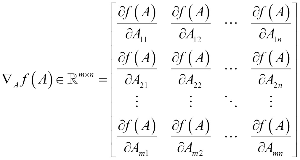
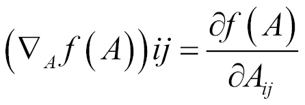
Gradient for functions with respect to a real-valued matrixA is defined as the matrix of partial derivatives of A and is denoted as follows:

TensorFlow does not do numerical differentiation; rather, it supports automatic differentiation. By specifying operations in a TensorFlow graph, it can automatically run the chain rule through the graph and, as it knows the derivatives of each operation we specify, it can combine them automatically.

The following example shows training a network using MNIST data, the MNIST database consists of handwritten digits. It has a training set of 60,000 examples and a test set of 10,000 samples. The digits are size-normalized.

Here backpropagation is performed without any API usage and derivatives are calculated manually. We get 913 correct out of 1,000 tests. This concept will be introduced in the next chapter.

The following code snippet describes how to get the mnist dataset and initialize weights and biases:

import tensorflow as tf

# get mnist dataset
from tensorflow.examples.tutorials.mnist import input_data
data = input_data.read_data_sets("MNIST_data/", one_hot=True)

# x represents image with 784 values as columns (28*28), y represents output digit
x = tf.placeholder(tf.float32, [None, 784])
y = tf.placeholder(tf.float32, [None, 10])

# initialize weights and biases [w1,b1][w2,b2]
numNeuronsInDeepLayer = 30
w1 = tf.Variable(tf.truncated_normal([784, numNeuronsInDeepLayer]))
b1 = tf.Variable(tf.truncated_normal([1, numNeuronsInDeepLayer]))
w2 = tf.Variable(tf.truncated_normal([numNeuronsInDeepLayer, 10]))
b2 = tf.Variable(tf.truncated_normal([1, 10]))

We now define a two-layered network with a nonlinear sigmoid function; a squared loss function is applied and optimized using a backward propagation algorithm, as shown in the following snippet:

# non-linear sigmoid function at each neuron
def sigmoid(x):
    sigma = tf.div(tf.constant(1.0), tf.add(tf.constant(1.0), tf.exp(tf.negative(x))))
    return sigma

# starting from first layer with wx+b, then apply sigmoid to add non-linearity
z1 = tf.add(tf.matmul(x, w1), b1)
a1 = sigmoid(z1)
z2 = tf.add(tf.matmul(a1, w2), b2)
a2 = sigmoid(z2)

# calculate the loss (delta)
loss = tf.subtract(a2, y)

# derivative of the sigmoid function der(sigmoid)=sigmoid*(1-sigmoid)
def sigmaprime(x):
    return tf.multiply(sigmoid(x), tf.subtract(tf.constant(1.0), sigmoid(x)))

# backward propagation
dz2 = tf.multiply(loss, sigmaprime(z2))
db2 = dz2
dw2 = tf.matmul(tf.transpose(a1), dz2)

da1 = tf.matmul(dz2, tf.transpose(w2))
dz1 = tf.multiply(da1, sigmaprime(z1))
db1 = dz1
dw1 = tf.matmul(tf.transpose(x), dz1)

# finally update the network
eta = tf.constant(0.5)
step = [
    tf.assign(w1,
              tf.subtract(w1, tf.multiply(eta, dw1)))
    , tf.assign(b1,
                tf.subtract(b1, tf.multiply(eta,
                                             tf.reduce_mean(db1, axis=[0]))))
    , tf.assign(w2,
                tf.subtract(w2, tf.multiply(eta, dw2)))
    , tf.assign(b2,
                tf.subtract(b2, tf.multiply(eta,
                                             tf.reduce_mean(db2, axis=[0]))))
]

acct_mat = tf.equal(tf.argmax(a2, 1), tf.argmax(y, 1))
acct_res = tf.reduce_sum(tf.cast(acct_mat, tf.float32))

sess = tf.InteractiveSession()
sess.run(tf.global_variables_initializer())

for i in range(10000):
    batch_xs, batch_ys = data.train.next_batch(10)
    sess.run(step, feed_dict={x: batch_xs,
                              y: batch_ys})
    if i % 1000 == 0:
        res = sess.run(acct_res, feed_dict=
        {x: data.test.images[:1000],
         y: data.test.labels[:1000]})
        print(res)

The output of this is shown as follows:

Extracting MNIST_data
125.0
814.0
870.0
874.0
889.0
897.0
906.0
903.0
922.0
913.0

Now, let's use automatic differentiation with TensorFlow. The following example demonstrates the use of GradientDescentOptimizer. We get 924 correct out of 1,000 tests.

import tensorflow as tf

# get mnist dataset
from tensorflow.examples.tutorials.mnist import input_data
data = input_data.read_data_sets("MNIST_data/", one_hot=True)

# x represents image with 784 values as columns (28*28), y represents output digit
x = tf.placeholder(tf.float32, [None, 784])
y = tf.placeholder(tf.float32, [None, 10])

# initialize weights and biases [w1,b1][w2,b2]
numNeuronsInDeepLayer = 30
w1 = tf.Variable(tf.truncated_normal([784, numNeuronsInDeepLayer]))
b1 = tf.Variable(tf.truncated_normal([1, numNeuronsInDeepLayer]))
w2 = tf.Variable(tf.truncated_normal([numNeuronsInDeepLayer, 10]))
b2 = tf.Variable(tf.truncated_normal([1, 10]))

# non-linear sigmoid function at each neuron
def sigmoid(x):
    sigma = tf.div(tf.constant(1.0), tf.add(tf.constant(1.0), tf.exp(tf.negative(x))))
    return sigma

# starting from first layer with wx+b, then apply sigmoid to add non-linearity
z1 = tf.add(tf.matmul(x, w1), b1)
a1 = sigmoid(z1)
z2 = tf.add(tf.matmul(a1, w2), b2)
a2 = sigmoid(z2)

# calculate the loss (delta)
loss = tf.subtract(a2, y)

# derivative of the sigmoid function der(sigmoid)=sigmoid*(1-sigmoid)
def sigmaprime(x):
    return tf.multiply(sigmoid(x), tf.subtract(tf.constant(1.0), sigmoid(x)))

# automatic differentiation
cost = tf.multiply(loss, loss)
step = tf.train.GradientDescentOptimizer(0.1).minimize(cost)

acct_mat = tf.equal(tf.argmax(a2, 1), tf.argmax(y, 1))
acct_res = tf.reduce_sum(tf.cast(acct_mat, tf.float32))

sess = tf.InteractiveSession()
sess.run(tf.global_variables_initializer())

for i in range(10000):
    batch_xs, batch_ys = data.train.next_batch(10)
    sess.run(step, feed_dict={x: batch_xs,
                              y: batch_ys})
    if i % 1000 == 0:
        res = sess.run(acct_res, feed_dict=
        {x: data.test.images[:1000],
         y: data.test.labels[:1000]})
        print(res)

The output of this is shown as follows:

96.0
 777.0
 862.0
 870.0
 889.0
 901.0
 911.0
 905.0
 914.0
 924.0

The following example shows linear regression using gradient descent:

import tensorflow as tf
import numpy
import matplotlib.pyplot as plt
rndm = numpy.random

# config parameters
learningRate = 0.01
trainingEpochs = 1000
displayStep = 50

# create the training data
trainX = numpy.asarray([3.3,4.4,5.5,6.71,6.93,4.168,9.779,6.182,7.59,2.167,
                         7.042,10.791,5.313,7.997,5.654,9.27,3.12])
trainY = numpy.asarray([1.7,2.76,2.09,3.19,1.694,1.573,3.366,2.596,2.53,1.221,
                         2.827,3.465,1.65,2.904,2.42,2.94,1.34])
nSamples = trainX.shape[0]

# tf inputs
X = tf.placeholder("float")
Y = tf.placeholder("float")

# initialize weights and bias
W = tf.Variable(rndm.randn(), name="weight")
b = tf.Variable(rndm.randn(), name="bias")

# linear model
linearModel = tf.add(tf.multiply(X, W), b)

# mean squared error
loss = tf.reduce_sum(tf.pow(linearModel-Y, 2))/(2*nSamples)

# Gradient descent
opt = tf.train.GradientDescentOptimizer(learningRate).minimize(loss)

# initializing variables
init = tf.global_variables_initializer()

# run
with tf.Session() as sess:
    sess.run(init)

    # fitting the training data
    for epoch in range(trainingEpochs):
        for (x, y) in zip(trainX, trainY):
            sess.run(opt, feed_dict={X: x, Y: y})

        # print logs
        if (epoch+1) % displayStep == 0:
            c = sess.run(loss, feed_dict={X: trainX, Y:trainY})
            print("Epoch is:", '%04d' % (epoch+1), "loss=", "{:.9f}".format(c), "W=", sess.run(W), "b=", sess.run(b))

    print("optimization done...")
    trainingLoss = sess.run(loss, feed_dict={X: trainX, Y: trainY})
    print("Training loss=", trainingLoss, "W=", sess.run(W), "b=", sess.run(b), '\n')

    # display the plot
    plt.plot(trainX, trainY, 'ro', label='Original data')
    plt.plot(trainX, sess.run(W) * trainX + sess.run(b), label='Fitted line')
    plt.legend()
    plt.show()

    # Testing example, as requested (Issue #2)
    testX = numpy.asarray([6.83, 4.668, 8.9, 7.91, 5.7, 8.7, 3.1, 2.1])
    testY = numpy.asarray([1.84, 2.273, 3.2, 2.831, 2.92, 3.24, 1.35, 1.03])

    print("Testing... (Mean square loss Comparison)")
    testing_cost = sess.run(
        tf.reduce_sum(tf.pow(linearModel - Y, 2)) / (2 * testX.shape[0]),
        feed_dict={X: testX, Y: testY})
    print("Testing cost=", testing_cost)
    print("Absolute mean square loss difference:", abs(trainingLoss - testing_cost))

    plt.plot(testX, testY, 'bo', label='Testing data')
    plt.plot(trainX, sess.run(W) * trainX + sess.run(b), label='Fitted line')
    plt.legend()
    plt.show()

The output of this is shown as follows:

Epoch is: 0050 loss= 0.141912043 W= 0.10565 b= 1.8382
 Epoch is: 0100 loss= 0.134377643 W= 0.11413 b= 1.7772
 Epoch is: 0150 loss= 0.127711013 W= 0.122106 b= 1.71982
 Epoch is: 0200 loss= 0.121811897 W= 0.129609 b= 1.66585
 Epoch is: 0250 loss= 0.116592340 W= 0.136666 b= 1.61508
 Epoch is: 0300 loss= 0.111973859 W= 0.143304 b= 1.56733
 Epoch is: 0350 loss= 0.107887231 W= 0.149547 b= 1.52241
 Epoch is: 0400 loss= 0.104270980 W= 0.15542 b= 1.48017
 Epoch is: 0450 loss= 0.101070963 W= 0.160945 b= 1.44043
 Epoch is: 0500 loss= 0.098239250 W= 0.166141 b= 1.40305
 Epoch is: 0550 loss= 0.095733419 W= 0.171029 b= 1.36789
 Epoch is: 0600 loss= 0.093516059 W= 0.175626 b= 1.33481
 Epoch is: 0650 loss= 0.091553882 W= 0.179951 b= 1.3037
 Epoch is: 0700 loss= 0.089817807 W= 0.184018 b= 1.27445
 Epoch is: 0750 loss= 0.088281371 W= 0.187843 b= 1.24692
 Epoch is: 0800 loss= 0.086921677 W= 0.191442 b= 1.22104
 Epoch is: 0850 loss= 0.085718453 W= 0.194827 b= 1.19669
 Epoch is: 0900 loss= 0.084653646 W= 0.198011 b= 1.17378
 Epoch is: 0950 loss= 0.083711281 W= 0.201005 b= 1.15224
 Epoch is: 1000 loss= 0.082877308 W= 0.203822 b= 1.13198
 optimization done...
 Training loss= 0.0828773 W= 0.203822 b= 1.13198
Testing... (Mean square loss Comparison)
 Testing cost= 0.0957726
 Absolute mean square loss difference: 0.0128952

The plots are as follows:

The following image shows the fitted line on testing data using the model:

Gradient is the first derivative for functions of vectors, whereas hessian is the second derivative. We will go through the notation now:

Similar to the gradient, the hessian is defined only when f(x) is real-valued.

Note

The algebraic function used is

.

The following example shows the hessian implementation using TensorFlow:

import tensorflow as tf
import numpy as np

X = tf.Variable(np.random.random_sample(), dtype=tf.float32)
y = tf.Variable(np.random.random_sample(), dtype=tf.float32)

def createCons(x):
    return tf.constant(x, dtype=tf.float32)

function = tf.pow(X, createCons(2)) + createCons(2) * X * y + createCons(3) * tf.pow(y, createCons(2)) + createCons(4) * X + createCons(5) * y + createCons(6)

# compute hessian
def hessian(func, varbles):
    matrix = []
    for v_1 in varbles:
        tmp = []
        for v_2 in varbles:
            # calculate derivative twice, first w.r.t v2 and then w.r.t v1
            tmp.append(tf.gradients(tf.gradients(func, v_2)[0], v_1)[0])
        tmp = [createCons(0) if t == None else t for t in tmp]
        tmp = tf.stack(tmp)
        matrix.append(tmp)
    matrix = tf.stack(matrix)
    return matrix

hessian = hessian(function, [X, y])

sess = tf.Session()
sess.run(tf.initialize_all_variables())
print(sess.run(hessian))

The output of this is shown as follows:

 [[ 2.  2.] [ 2.  6.]]

Determinant shows us information about the matrix that is helpful in linear equations and also helps in finding the inverse of a matrix.

For a given matrix X, the determinant is shown as follows:

The following example shows how to get a determinant using TensorFlow:

import tensorflow as tf
import numpy as np

x = np.array([[10.0, 15.0, 20.0], [0.0, 1.0, 5.0], [3.0, 5.0, 7.0]], dtype=np.float32)

det = tf.matrix_determinant(x)

with tf.Session() as sess:
    print(sess.run(det))

The output of this is shown as follows:

-15.0

We will study AdamOptimizer here; TensorFlow AdamOptimizer uses Kingma and Ba's Adam algorithm to manage the learning rate. Adam has many advantages over the simple GradientDescentOptimizer. The first is that it uses moving averages of the parameters, which enables Adam to use a larger step size, and it will converge to this step size without any fine-tuning.

The disadvantage of Adam is that it requires more computation to be performed for each parameter in each training step. GradientDescentOptimizer can be used as well, but it would require more hyperparameter tuning before it would converge as quickly. The following example shows how to use AdamOptimizer:

Here, automatic differentiation computes gradients without user input:

import numpy as np
import seaborn
import matplotlib.pyplot as plt
import tensorflow as tf

# input dataset
xData = np.arange(100, step=.1)
yData = xData + 20 * np.sin(xData/10)

# scatter plot for input data
plt.scatter(xData, yData)
plt.show()

# defining data size and batch size
nSamples = 1000
batchSize = 100

# resize
xData = np.reshape(xData, (nSamples,1))
yData = np.reshape(yData, (nSamples,1))

# input placeholders
x = tf.placeholder(tf.float32, shape=(batchSize, 1))
y = tf.placeholder(tf.float32, shape=(batchSize, 1))

# init weight and bias
with tf.variable_scope("linearRegression"):
 W = tf.get_variable("weights", (1, 1), initializer=tf.random_normal_initializer())
 b = tf.get_variable("bias", (1,), initializer=tf.constant_initializer(0.0))

 y_pred = tf.matmul(x, W) + b
 loss = tf.reduce_sum((y - y_pred)**2/nSamples)

# optimizer
opt = tf.train.AdamOptimizer().minimize(loss)
with tf.Session() as sess:
    sess.run(tf.global_variables_initializer())

    # gradient descent loop for 500 steps
    for _ in range(500):
     # random minibatch
     indices = np.random.choice(nSamples, batchSize)

     X_batch, y_batch = xData[indices], yData[indices]

     # gradient descent step
     _, loss_val = sess.run([opt, loss], feed_dict={x: X_batch, y: y_batch})

Here is the scatter plot for the dataset:

This is the plot of the learned model on the data: