


 Download code from GitHub
TensorFlow 101
TensorFlow is one of the popular libraries for solving problems with machine learning and deep learning. After being developed for internal use by Google, it was released for public use and development as open source. Let us understand the three models of the TensorFlow: data model, programming model, and execution model.
TensorFlow data model consists of tensors, and the programming model consists of data flow graphs or computation graphs. TensorFlow execution model consists of firing the nodes in a sequence based on the dependence conditions, starting from the initial nodes that depend on inputs.
In this chapter, we will review the elements of TensorFlow that make up these three models, also known as the core TensorFlow.
We will cover the following topics in this chapter:
- TensorFlow core
- Tensors
- Constants
- Placeholders
- Operations
- Creating tensors from Python objects
- Variables
- Tensors generated from library functions
- Data flow graph or computation graph
- Order of execution and lazy loading
- Executing graphs across compute devices - CPU and GPGPU
- Multiple graphs
- TensorBoard overview
What is TensorFlow?
According to the TensorFlow website (www.tensorflow.org):
Initially developed by Google for its internal consumption, it was released as open source on November 9, 2015. Since then, TensorFlow has been extensively used to develop machine learning and deep neural network models in various domains and continues to be used within Google for research and product development. TensorFlow 1.0 was released on February 15, 2017. Makes one wonder if it was a Valentine's Day gift from Google to machine learning engineers!
TensorFlow can be described with a data model, a programming model, and an execution model:
- Data model comprises of tensors, that are the basic data units created, manipulated, and saved in a TensorFlow program.
- Programming model comprises of data flow graphs or computation graphs. Creating a program in TensorFlow means building one or more TensorFlow computation graphs.
- Execution model consists of firing the nodes of a computation graph in a sequence of dependence. The execution starts by running the nodes that are directly connected to inputs and only depend on inputs being present.
To use TensorFlow in your projects, you need to learn how to program using the TensorFlow API. TensorFlow has multiple APIs that can be used to interact with the library. The TF APIs or libraries are divided into two levels:
- Lower-level library: The lower level library, also known as TensorFlow core, provides very fine-grained lower level functionality, thereby offering complete control on how to use and implement the library in the models. We will cover TensorFlow core in this chapter.
- Higher-level libraries: These libraries provide high-level functionalities and are comparatively easier to learn and implement in the models. Some of the libraries include TF Estimators, TFLearn, TFSlim, Sonnet, and Keras. We will cover some of these libraries in the next chapter.
TensorFlow core
TensorFlow core is the lower level library on which the higher level TensorFlow modules are built. The concepts of the lower level library are very important to learn before we go deeper into learning the advanced TensorFlow. In this section, we will have a quick recap of all those core concepts.
Code warm-up - Hello TensorFlow
As a customary tradition when learning any new programming language, library, or platform, let's write the simple Hello TensorFlow code as a warm-up exercise before we dive deeper.
Open the file ch-01_TensorFlow_101.ipynb in Jupyter Notebook to follow and run the code as you study the text.
- Import the TensorFlow Library with the following code:
import tensorflow as tf
- Get a TensorFlow session. TensorFlow offers two kinds of sessions: Session() and InteractiveSession(). We will create an interactive session with the following code:
tfs = tf.InteractiveSession()
- Define a TensorFlow constant, hello:
hello = tf.constant("Hello TensorFlow !!")
- Execute the constant in a TensorFlow session and print the output:
print(tfs.run(hello))
- You will get the following output:
'Hello TensorFlow !!'
Now that you have written and executed the first two lines of code with TensorFlow, let's look at the basic ingredients of TensorFlow.
Tensors
Tensors are the basic elements of computation and a fundamental data structure in TensorFlow. Probably the only data structure that you need to learn to use TensorFlow. A tensor is an n-dimensional collection of data, identified by rank, shape, and type.
Rank is the number of dimensions of a tensor, and shape is the list denoting the size in each dimension. A tensor can have any number of dimensions. You may be already familiar with quantities that are a zero-dimensional collection (scalar), a one-dimensional collection (vector), a two-dimensional collection (matrix), and a multidimensional collection.
A scalar value is a tensor of rank 0 and thus has a shape of [1]. A vector or a one-dimensional array is a tensor of rank 1 and has a shape of [columns] or [rows]. A matrix or a two-dimensional array is a tensor of rank 2 and has a shape of [rows, columns]. A three-dimensional array would be a tensor of rank 3, and in the same manner, an n-dimensional array would be a tensor of rank n.
- Tensors page on Wikipedia, at https://en.wikipedia.org/wiki/Tensor
- Introduction to Tensors guide from NASA, at https://www.grc.nasa.gov/www/k-12/Numbers/Math/documents/Tensors_TM2002211716.pdf
A tensor can store data of one type in all its dimensions, and the data type of its elements is known as the data type of the tensor.
At the time of writing this book, the TensorFlow had the following data types defined:
| TensorFlow Python API data type | Description |
| tf.float16 | 16-bit half-precision floating point |
| tf.float32 | 32-bit single-precision floating point |
| tf.float64 | 64-bit double-precision floating point |
| tf.bfloat16 | 16-bit truncated floating point |
| tf.complex64 | 64-bit single-precision complex |
| tf.complex128 | 128-bit double-precision complex |
| tf.int8 | 8-bit signed integer |
| tf.uint8 | 8-bit unsigned integer |
| tf.uint16 | 16-bit unsigned integer |
| tf.int16 | 16-bit signed integer |
| tf.int32 | 32-bit signed integer |
| tf.int64 | 64-bit signed integer |
| tf.bool | Boolean |
| tf.string | String |
| tf.qint8 | Quantized 8-bit signed integer |
| tf.quint8 | Quantized 8-bit unsigned integer |
| tf.qint16 | Quantized 16-bit signed integer |
| tf.quint16 | Quantized 16-bit unsigned integer |
| tf.qint32 | Quantized 32-bit signed integer |
| tf.resource | Handle to a mutable resource |
Tensors can be created in the following ways:
- By defining constants, operations, and variables, and passing the values to their constructor.
- By defining placeholders and passing the values to session.run().
- By converting Python objects such as scalar values, lists, and NumPy arrays with the tf.convert_to_tensor() function.
Let's examine different ways of creating Tensors.
Constants
The constant valued tensors are created using the tf.constant() function that has the following signature:
tf.constant(
  value,
  dtype=None,
  shape=None,
  name='Const',
  verify_shape=False
)
Let's look at the example code provided in the Jupyter Notebook with this book:
c1=tf.constant(5,name='x')
c2=tf.constant(6.0,name='y')
c3=tf.constant(7.0,tf.float32,name='z')
Let's look into the code in detail:
- The first line defines a constant tensor c1, gives it value 5, and names it x.
- The second line defines a constant tensor c2, stores value 6.0, and names it y.
- When we print these tensors, we see that the data types of c1 and c2 are automatically deduced by TensorFlow.
- To specifically define a data type, we can use the dtype parameter or place the data type as the second argument. In the preceding code example, we define the data type as tf.float32 for c3.
Let's print the constants c1, c2, and c3:
print('c1 (x): ',c1)
print('c2 (y): ',c2)
print('c3 (z): ',c3)
When we print these constants, we get the following output:
c1 (x):  Tensor("x:0", shape=(), dtype=int32)
c2 (y):  Tensor("y:0", shape=(), dtype=float32)
c3 (z):  Tensor("z:0", shape=(), dtype=float32)
In order to print the values of these constants, we have to execute them in a TensorFlow session with the tfs.run() command:
print('run([c1,c2,c3]) : ',tfs.run([c1,c2,c3]))
We see the following output:
run([c1,c2,c3]) : [5, 6.0, 7.0]
Operations
TensorFlow provides us with many operations that can be applied on Tensors. An operation is defined by passing values and assigning the output to another tensor. For example, in the provided Jupyter Notebook file, we define two operations, op1 and op2:
op1 = tf.add(c2,c3)
op2 = tf.multiply(c2,c3)
When we print op1 and op2, we find that they are defined as Tensors:
print('op1 : ', op1)
print('op2 : ', op2)
The output is as follows:
To print the value of these operations, we have to run them in our TensorFlow session:
print('run(op1) : ', tfs.run(op1))
print('run(op2) : ', tfs.run(op2))
The output is as follows:
run(op1) :  13.0
run(op2) :  42.0
The following table lists some of the built-in operations:
| Operation types | Operations |
| Arithmetic operations |
tf.add, tf.subtract, tf.multiply, tf.scalar_mul, tf.div, tf.divide, tf.truediv, tf.floordiv, tf.realdiv, tf.truncatediv, tf.floor_div, tf.truncatemod, tf.floormod, tf.mod, tf.cross |
| Basic math operations |
tf.add_n, tf.abs, tf.negative, tf.sign, tf.reciprocal, tf.square, tf.round, tf.sqrt, tf.rsqrt, tf.pow, tf.exp, tf.expm1, tf.log, tf.log1p, tf.ceil, tf.floor, tf.maximum, tf.minimum, tf.cos, tf.sin, tf.lbeta, tf.tan, tf.acos, tf.asin, tf.atan, tf.lgamma, tf.digamma, tf.erf, tf.erfc, tf.igamma, tf.squared_difference, tf.igammac, tf.zeta, tf.polygamma, tf.betainc, tf.rint |
| Matrix math operations |
tf.diag, tf.diag_part, tf.trace, tf.transpose, tf.eye, tf.matrix_diag, tf.matrix_diag_part, tf.matrix_band_part, tf.matrix_set_diag, tf.matrix_transpose, tf.matmul, tf.norm, tf.matrix_determinant, tf.matrix_inverse, tf.cholesky, tf.cholesky_solve, tf.matrix_solve, tf.matrix_triangular_solve, tf.matrix_solve_ls, tf.qr, tf.self_adjoint_eig, tf.self_adjoint_eigvals, tf.svd |
| Tensor math operations | tf.tensordot |
| Complex number operations | tf.complex, tf.conj, tf.imag, tf.real |
| String operations |
tf.string_to_hash_bucket_fast, tf.string_to_hash_bucket_strong, tf.as_string, tf.encode_base64, tf.decode_base64, tf.reduce_join, tf.string_join, tf.string_split, tf.substr, tf.string_to_hash_bucket |
Placeholders
While constants allow us to provide a value at the time of defining the tensor, the placeholders allow us to create tensors whose values can be provided at runtime. TensorFlow provides the tf.placeholder() function with the following signature to create placeholders:
tf.placeholder(
  dtype,
  shape=None,
  name=None
  )
As an example, let's create two placeholders and print them:
p1 = tf.placeholder(tf.float32)
p2 = tf.placeholder(tf.float32)
print('p1 : ', p1)
print('p2 : ', p2)
We see the following output:
p1 :  Tensor("Placeholder:0", dtype=float32)
p2 :  Tensor("Placeholder_1:0", dtype=float32)
Now let's define an operation using these placeholders:
op4 = p1 * p2
TensorFlow allows using shorthand symbols for various operations. In the earlier example, p1 * p2 is shorthand for tf.multiply(p1,p2):
print('run(op4,{p1:2.0, p2:3.0}) : ',tfs.run(op4,{p1:2.0, p2:3.0}))
The preceding command runs the op4 in the TensorFlow Session, feeding the Python dictionary (the second argument to the run() operation) with values for p1 and p2.
The output is as follows:
run(op4,{p1:2.0, p2:3.0}) : 6.0
We can also specify the dictionary using the feed_dict parameter in the run() operation:
print('run(op4,feed_dict = {p1:3.0, p2:4.0}) : ',
      tfs.run(op4, feed_dict={p1: 3.0, p2: 4.0}))
The output is as follows:
run(op4,feed_dict = {p1:3.0, p2:4.0}) : 12.0
Let's look at one last example, with a vector being fed to the same operation:
print('run(op4,feed_dict = {p1:[2.0,3.0,4.0], p2:[3.0,4.0,5.0]}) : ',
    tfs.run(op4,feed_dict = {p1:[2.0,3.0,4.0], p2:[3.0,4.0,5.0]}))
The output is as follows:
run(op4,feed_dict={p1:[2.0,3.0,4.0],p2:[3.0,4.0,5.0]}):[ 6. 12. 20.]
The elements of the two input vectors are multiplied in an element-wise fashion.
Creating tensors from Python objects
We can create tensors from Python objects such as lists and NumPy arrays, using the tf.convert_to_tensor() operation with the following signature:
tf.convert_to_tensor(
  value,
  dtype=None,
  name=None,
  preferred_dtype=None
  )
Let's create some tensors and print them for practice:
- Create and print a 0-D Tensor:
tf_t=tf.convert_to_tensor(5.0,dtype=tf.float64)

print('tf_t : ',tf_t)
print('run(tf_t) : ',tfs.run(tf_t))
The output is as follows:
tf_t :  Tensor("Const_1:0", shape=(), dtype=float64)
run(tf_t) : 5.0
- Create and print a 1-D Tensor:
a1dim = np.array([1,2,3,4,5.99])
print("a1dim Shape : ",a1dim.shape)

tf_t=tf.convert_to_tensor(a1dim,dtype=tf.float64)

print('tf_t : ',tf_t)
print('tf_t[0] : ',tf_t[0])
print('tf_t[0] : ',tf_t[2])
print('run(tf_t) : \n',tfs.run(tf_t))
The output is as follows:
a1dim Shape :  (5,)
tf_t :  Tensor("Const_2:0", shape=(5,), dtype=float64)
tf_t[0] :  Tensor("strided_slice:0", shape=(), dtype=float64)
tf_t[0] :  Tensor("strided_slice_1:0", shape=(), dtype=float64)
run(tf_t) :
 [ 1.    2.    3.    4.    5.99]
- Create and print a 2-D Tensor:
a2dim = np.array([(1,2,3,4,5.99),
                  (2,3,4,5,6.99),
                  (3,4,5,6,7.99)
                 ])
print("a2dim Shape : ",a2dim.shape)

tf_t=tf.convert_to_tensor(a2dim,dtype=tf.float64)

print('tf_t : ',tf_t)
print('tf_t[0][0] : ',tf_t[0][0])
print('tf_t[1][2] : ',tf_t[1][2])
print('run(tf_t) : \n',tfs.run(tf_t))
The output is as follows:
- Create and print a 3-D Tensor:
a3dim = np.array([[[1,2],[3,4]],
                  [[5,6],[7,8]]
                 ])
print("a3dim Shape : ",a3dim.shape)

tf_t=tf.convert_to_tensor(a3dim,dtype=tf.float64)

print('tf_t : ',tf_t)
print('tf_t[0][0][0] : ',tf_t[0][0][0])
print('tf_t[1][1][1] : ',tf_t[1][1][1])
print('run(tf_t) : \n',tfs.run(tf_t))
The output is as follows:
a3dim Shape :  (2, 2, 2)
tf_t :  Tensor("Const_4:0", shape=(2, 2, 2), dtype=float64)
tf_t[0][0][0] :  Tensor("strided_slice_8:0", shape=(), dtype=float64)
tf_t[1][1][1] :  Tensor("strided_slice_11:0", shape=(), dtype=float64)
run(tf_t) :
 [[[ 1.  2.][ 3.  4.]]
  [[ 5.  6.][ 7.  8.]]]
Variables
So far, we have seen how to create tensor objects of various kinds: constants, operations, and placeholders. While working with TensorFlow to build and train models, you will often need to hold the values of parameters in a memory location that can be updated at runtime. That memory location is identified by variables in TensorFlow.
In TensorFlow, variables are tensor objects that hold values that can be modified during the execution of the program.
While tf.Variable appears similar to tf.placeholder, there are subtle differences between the two:
| tf.placeholder | tf.Variable |
| tf.placeholder defines input data that does not change over time | tf.Variable defines variable values that are modified over time |
| tf.placeholder does not need an initial value at the time of definition | tf.Variable needs an initial value at the time of definition |
In TensorFlow, a variable can be created with tf.Variable(). Let's see an example of placeholders and variables with a linear model:

- We define the model parameters w and b as variables with initial values of [.3] and [-0.3], respectively:
w = tf.Variable([.3], tf.float32)
b = tf.Variable([-.3], tf.float32)
- The input x is defined as a placeholder and the output y is defined as an operation:
x = tf.placeholder(tf.float32)
y = w * x + b
- Let's print w, v, x, and y and see what we get:
print("w:",w)
print("x:",x)
print("b:",b)
print("y:",y)
We get the following output:
w: <tf.Variable 'Variable:0' shape=(1,) dtype=float32_ref>
x: Tensor("Placeholder_2:0", dtype=float32)
b: <tf.Variable 'Variable_1:0' shape=(1,) dtype=float32_ref>
y: Tensor("add:0", dtype=float32)
The output shows that x is a placeholder tensor and y is an operation tensor, while w and b are variables with shape (1,) and data type float32.
Before you can use the variables in a TensorFlow session, they have to be initialized. You can initialize a single variable by running its initializer operation.
For example, let's initialize the variable w:
tfs.run(w.initializer)
However, in practice, we use a convenience function provided by the TensorFlow to initialize all the variables:
tfs.run(tf.global_variables_initializer())
The global initializer convenience function can also be invoked in the following manner, instead of being invoked inside the run() function of a session object:
tf.global_variables_initializer().run()
After initializing the variables, let's run our model to give the output for values of x = [1,2,3,4]:
print('run(y,{x:[1,2,3,4]}) : ',tfs.run(y,{x:[1,2,3,4]}))
We get the following output:
run(y,{x:[1,2,3,4]}) : [ 0. 0.30000001 0.60000002 0.90000004]
Tensors generated from library functions
Tensors can also be generated from various TensorFlow functions. These generated tensors can either be assigned to a constant or a variable, or provided to their constructor at the time of initialization.
As an example, the following code generates a vector of 100 zeroes and prints it:
a=tf.zeros((100,))
print(tfs.run(a))
TensorFlow provides different types of functions to populate the tensors at the time of their definition:
- Populating all elements with the same values
- Populating elements with sequences
- Populating elements with a random probability distribution, such as the normal distribution or the uniform distribution
Populating tensor elements with the same values
The following table lists some of the tensor generating library functions to populate all the elements of the tensor with the same values:
| Tensor generating function | Description |
zeros( |
Creates a tensor of the provided shape, with all elements set to zero |
zeros_like( |
Creates a tensor of the same shape as the argument, with all elements set to zero |
ones( |
Creates a tensor of the provided shape, with all elements set to one |
ones_like( |
Creates a tensor of the same shape as the argument, with all elements set to one |
fill( |
Creates a tensor of the shape as the dims argument, with all elements set to value; for example, a = tf.fill([100],0) |
Populating tensor elements with sequences
The following table lists some of the tensor generating functions to populate elements of the tensor with sequences:
| Tensor generating function | Description |
lin_space( |
Generates a 1-D tensor from a sequence of num numbers within the range [start, stop]. The tensor has the same data type as the start argument. For example, a = tf.lin_space(1,100,10) generates a tensor with values [1,12,23,34,45,56,67,78,89,100]. |
range( |
Generates a 1-D tensor from a sequence of numbers within the range [start, limit], with the increments of delta. If the dtype argument is not specified, then the tensor has the same data type as the start argument. This function comes in two versions. In the second version, if the start argument is omitted, then start becomes number 0. For example, a = tf.range(1,91,10) generates a tensor with values [1,11,21,31,41,51,61,71,81]. Note that the value of the limit argument, that is 91, is not included in the final generated sequence. |
Populating tensor elements with a random distribution
TensorFlow provides us with the functions to generate tensors filled with random valued distributions.
The distributions generated are affected by the graph-level or the operation-level seed. The graph-level seed is set using tf.set_random_seed, while the operation-level seed is given as the argument seed in all of the random distribution functions. If no seed is specified, then a random seed is used.
The following table lists some of the tensor generating functions to populate elements of the tensor with random valued distributions:
| Tensor generating function | Description |
random_normal( |
Generates a tensor of the specified shape, filled with values from a normal distribution: normal(mean, stddev). |
truncated_normal( |
Generates a tensor of the specified shape, filled with values from a truncated normal distribution: normal(mean, stddev). Truncated means that the values returned are always at a distance less than two standard deviations from the mean. |
random_uniform( |
Generates a tensor of the specified shape, filled with values from a uniform distribution: uniform([minval, maxval)). |
random_gamma(
|
Generates tensors of the specified shape, filled with values from gamma distributions: gamma(alpha,beta). More details on the random_gamma function can be found at the following link: https://www.tensorflow.org/api_docs/python/tf/random_gamma. |
Getting Variables with tf.get_variable()
If you define a variable with a name that has been defined before, then TensorFlow throws an exception. Hence, it is convenient to use the tf.get_variable() function instead of tf.Variable(). The function tf.get_variable() returns the existing variable with the same name if it exists, and creates the variable with the specified shape and initializer if it does not exist. For example:
w = tf.get_variable(name='w',shape=[1],dtype=tf.float32,initializer=[.3])
b = tf.get_variable(name='b',shape=[1],dtype=tf.float32,initializer=[-.3])
The initializer can be a tensor or list of values as shown in above examples or one of the inbuilt initializers:
- tf.constant_initializer
- tf.random_normal_initializer
- tf.truncated_normal_initializer
- tf.random_uniform_initializer
- tf.uniform_unit_scaling_initializer
- tf.zeros_initializer
- tf.ones_initializer
- tf.orthogonal_initializer
In distributed TensorFlow where we can run the code across machines, the tf.get_variable() gives us global variables. To get the local variables TensorFlow has a function with similar signature: tf.get_local_variable().
Sharing or Reusing Variables: Getting already-defined variables promotes reuse. However, an exception will be thrown if the reuse flags are not set by using tf.variable_scope.reuse_variable() or tf.variable.scope(reuse=True).
Now that you have learned how to define tensors, constants, operations, placeholders, and variables, let's learn about the next level of abstraction in TensorFlow, that combines these basic elements together to form a basic unit of computation, the data flow graph or computational graph.
Data flow graph or computation graph
A data flow graph or computation graph is the basic unit of computation in TensorFlow. We will refer to them as the computation graph from now on. A computation graph is made up of nodes and edges. Each node represents an operation (tf.Operation) and each edge represents a tensor (tf.Tensor) that gets transferred between the nodes.
A program in TensorFlow is basically a computation graph. You create the graph with nodes representing variables, constants, placeholders, and operations and feed it to TensorFlow. TensorFlow finds the first nodes that it can fire or execute. The firing of these nodes results in the firing of other nodes, and so on.
Thus, TensorFlow programs are made up of two kinds of operations on computation graphs:
- Building the computation graph
- Running the computation graph
The TensorFlow comes with a default graph. Unless another graph is explicitly specified, a new node gets implicitly added to the default graph. We can get explicit access to the default graph using the following command:
graph = tf.get_default_graph()
For example, if we want to define three inputs and add them to produce output  , we can represent it using the following computation graph:
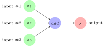
In TensorFlow, the add operation in the preceding image would correspond to the code y = tf.add( x1 + x2 + x3 ).
As we create the variables, constants, and placeholders, they get added to the graph. Then we create a session object to execute the operation objects and evaluate the tensor objects.
Let's build and execute a computation graph to calculate  , as we already saw in the preceding example:
# Assume Linear Model y = w * x + b
# Define model parameters
w = tf.Variable([.3], tf.float32)
b = tf.Variable([-.3], tf.float32)
# Define model input and output
x = tf.placeholder(tf.float32)
y = w * x + b
output = 0

with tf.Session() as tfs:
   # initialize and print the variable y
   tf.global_variables_initializer().run()
   output = tfs.run(y,{x:[1,2,3,4]})
print('output : ',output)
Creating and using a session in the with block ensures that the session is automatically closed when the block is finished. Otherwise, the session has to be explicitly closed with the tfs.close() command, where tfs is the session name.
Order of execution and lazy loading
The nodes are executed in the order of dependency. If node a depends on node b, then a will be executed before b when the execution of b is requested. A node is not executed unless either the node itself or another node depending on it is not requested for execution. This is also known as lazy loading; namely, the node objects are not created and initialized until they are needed.
Sometimes, you may want to control the order in which the nodes are executed in a graph. This can be achieved with the tf.Graph.control_dependencies() function. For example, if the graph has nodes a, b, c, and d and you want to execute c and d before a and b, then use the following statement:
with graph_variable.control_dependencies([c,d]):
  # other statements here
This makes sure that any node in the preceding with block is executed only after nodes c and d have been executed.
Executing graphs across compute devices - CPU and GPGPU
A graph can be divided into multiple parts and each part can be placed and executed on separate devices, such as a CPU or GPU. You can list all the devices available for graph execution with the following command:
from tensorflow.python.client import device_lib
print(device_lib.list_local_devices())
We get the following output (your output would be different, depending on the compute devices in your system):
[name: "/device:CPU:0"
device_type: "CPU"
memory_limit: 268435456
locality {
}
incarnation: 12900903776306102093
, name: "/device:GPU:0"
device_type: "GPU"
memory_limit: 611319808
locality {
  bus_id: 1
}
incarnation: 2202031001192109390
physical_device_desc: "device: 0, name: Quadro P5000, pci bus id: 0000:01:00.0, compute capability: 6.1"
]
The devices in TensorFlow are identified with the string /device:<device_type>:<device_idx>. In the above output, the CPU and GPU denote the device type and 0 denotes the device index.
One thing to note about the above output is that it shows only one CPU, whereas our computer has 8 CPUs. The reason for that is TensorFlow implicitly distributes the code across the CPU units and thus by default CPU:0 denotes all the CPU's available to TensorFlow. When TensorFlow starts executing graphs, it runs the independent paths within each graph in a separate thread, with each thread running on a separate CPU. We can restrict the number of threads used for this purpose by changing the number of inter_op_parallelism_threads. Similarly, if within an independent path, an operation is capable of running on multiple threads, TensorFlow will launch that specific operation on multiple threads. The number of threads in this pool can be changed by setting the number of intra_op_parallelism_threads.
Placing graph nodes on specific compute devices
Let us enable the logging of variable placement by defining a config object, set the log_device_placement property to true, and then pass this config object to the session as follows:
tf.reset_default_graph()

# Define model parameters
w = tf.Variable([.3], tf.float32)
b = tf.Variable([-.3], tf.float32)
# Define model input and output
x = tf.placeholder(tf.float32)
y = w * x + b

config = tf.ConfigProto()
config.log_device_placement=True

with tf.Session(config=config) as tfs:
   # initialize and print the variable y
   tfs.run(global_variables_initializer())
   print('output',tfs.run(y,{x:[1,2,3,4]}))
We get the following output in Jupyter Notebook console:
b: (VariableV2): /job:localhost/replica:0/task:0/device:GPU:0
b/read: (Identity): /job:localhost/replica:0/task:0/device:GPU:0
b/Assign: (Assign): /job:localhost/replica:0/task:0/device:GPU:0
w: (VariableV2): /job:localhost/replica:0/task:0/device:GPU:0
w/read: (Identity): /job:localhost/replica:0/task:0/device:GPU:0
mul: (Mul): /job:localhost/replica:0/task:0/device:GPU:0
add: (Add): /job:localhost/replica:0/task:0/device:GPU:0
w/Assign: (Assign): /job:localhost/replica:0/task:0/device:GPU:0
init: (NoOp): /job:localhost/replica:0/task:0/device:GPU:0
x: (Placeholder): /job:localhost/replica:0/task:0/device:GPU:0
b/initial_value: (Const): /job:localhost/replica:0/task:0/device:GPU:0
Const_1: (Const): /job:localhost/replica:0/task:0/device:GPU:0
w/initial_value: (Const): /job:localhost/replica:0/task:0/device:GPU:0
Const: (Const): /job:localhost/replica:0/task:0/device:GPU:0
Thus by default, the TensorFlow creates the variable and operations nodes on a device where it can get the highest performance. The variables and operations can be placed on specific devices by using tf.device() function. Let us place the graph on the CPU:
tf.reset_default_graph()

with tf.device('/device:CPU:0'):
    # Define model parameters
    w = tf.get_variable(name='w',initializer=[.3], dtype=tf.float32)
    b = tf.get_variable(name='b',initializer=[-.3], dtype=tf.float32)
    # Define model input and output
    x = tf.placeholder(name='x',dtype=tf.float32)
    y = w * x + b

config = tf.ConfigProto()
config.log_device_placement=True

with tf.Session(config=config) as tfs:
   # initialize and print the variable y
   tfs.run(tf.global_variables_initializer())
   print('output',tfs.run(y,{x:[1,2,3,4]}))
In the Jupyter console we see that now the variables have been placed on the CPU and the execution also takes place on the CPU:
b: (VariableV2): /job:localhost/replica:0/task:0/device:CPU:0
b/read: (Identity): /job:localhost/replica:0/task:0/device:CPU:0
b/Assign: (Assign): /job:localhost/replica:0/task:0/device:CPU:0
w: (VariableV2): /job:localhost/replica:0/task:0/device:CPU:0
w/read: (Identity): /job:localhost/replica:0/task:0/device:CPU:0
mul: (Mul): /job:localhost/replica:0/task:0/device:CPU:0
add: (Add): /job:localhost/replica:0/task:0/device:CPU:0
w/Assign: (Assign): /job:localhost/replica:0/task:0/device:CPU:0
init: (NoOp): /job:localhost/replica:0/task:0/device:CPU:0
x: (Placeholder): /job:localhost/replica:0/task:0/device:CPU:0
b/initial_value: (Const): /job:localhost/replica:0/task:0/device:CPU:0
Const_1: (Const): /job:localhost/replica:0/task:0/device:CPU:0
w/initial_value: (Const): /job:localhost/replica:0/task:0/device:CPU:0
Const: (Const): /job:localhost/replica:0/task:0/device:CPU:0
Simple placement
TensorFlow follows these simple rules, also known as the simple placement, for placing the variables on the devices:
If the graph was previously run,
    then the node is left on the device where it was placed earlier
Else If the tf.device() block is used,
    then the node is placed on the specified device
Else If the GPU is present
    then the node is placed on the first available GPU
Else If the GPU is not present
    then the node is placed on the CPU
Dynamic placement
The tf.device() can also be passed a function name instead of a device string. In such case, the function must return the device string. This feature allows complex algorithms for placing the variables on different devices. For example, TensorFlow provides a round robin device setter in tf.train.replica_device_setter() that we will discuss later in next section.
Soft placement
When you place a TensorFlow operation on the GPU, the TF must have the GPU implementation of that operation, known as the kernel. If the kernel is not present then the placement results in run-time error. Also if the GPU device you requested does not exist, you will get a run-time error. The best way to handle such errors is to allow the operation to be placed on the CPU if requesting the GPU device results in n error. This can be achieved by setting the following config value:
config.allow_soft_placement = True
GPU memory handling
When you start running the TensorFlow session, by default it grabs all of the GPU memory, even if you place the operations and variables only on one GPU in a multi-GPU system. If you try to run another session at the same time, you will get out of memory error. This can be solved in multiple ways:
- For multi-GPU systems, set the environment variable CUDA_VISIBLE_DEVICES=<list of device idx>
os.environ['CUDA_VISIBLE_DEVICES']='0'
The code executed after this setting will be able to grab all of the memory of only the visible GPU.
- When you do not want the session to grab all of the memory of the GPU, then you can use the config option per_process_gpu_memory_fraction to allocate a percentage of memory:
config.gpu_options.per_process_gpu_memory_fraction = 0.5
This will allocate 50% of the memory of all the GPU devices.
- You can also combine both of the above strategies, i.e. make only a percentage along with making only some of the GPU visible to the process.
- You can also limit the TensorFlow process to grab only the minimum required memory at the start of the process. As the process executes further, you can set a config option to allow the growth of this memory.
config.gpu_options.allow_growth = True
This option only allows for the allocated memory to grow, but the memory is never released back.
You will learn techniques for distributing computation across multiple compute devices and multiple nodes in later chapters.
Multiple graphs
You can create your own graphs separate from the default graph and execute them in a session. However, creating and executing multiple graphs is not recommended, as it has the following disadvantages:
- Creating and using multiple graphs in the same program would require multiple TensorFlow sessions and each session would consume heavy resources
- You cannot directly pass data in between graphs
Hence, the recommended approach is to have multiple subgraphs in a single graph. In case you wish to use your own graph instead of the default graph, you can do so with the tf.graph() command. Here is an example where we create our own graph, g, and execute it as the default graph:
g = tf.Graph()
output = 0

# Assume Linear Model y = w * x + b

with g.as_default():
 # Define model parameters
 w = tf.Variable([.3], tf.float32)
 b = tf.Variable([-.3], tf.float32)
 # Define model input and output
 x = tf.placeholder(tf.float32)
 y = w * x + b

with tf.Session(graph=g) as tfs:
 # initialize and print the variable y
 tf.global_variables_initializer().run()
 output = tfs.run(y,{x:[1,2,3,4]})

print('output : ',output)
TensorBoard
The complexity of a computation graph gets high even for moderately sized problems. Large computational graphs that represent complex machine learning models can become quite confusing and hard to understand. Visualization helps in easy understanding and interpretation of computation graphs, and thus accelerates the debugging and optimizations of TensorFlow programs. TensorFlow comes with a built-in tool that allows us to visualize computation graphs, namely, TensorBoard.
TensorBoard visualizes computation graph structure, provides statistical analysis and plots the values captured as summaries during the execution of computation graphs. Let's see how it works in practice.
A TensorBoard minimal example
- Start by defining the variables and placeholders for our linear model:
# Assume Linear Model y = w * x + b
# Define model parameters
w = tf.Variable([.3], name='w',dtype=tf.float32)
b = tf.Variable([-.3], name='b', dtype=tf.float32)
# Define model input and output
x = tf.placeholder(name='x',dtype=tf.float32)
y = w * x + b
- Initialize a session, and within the context of this session, do the following steps:
- Initialize global variables
- Create tf.summary.FileWriter that would create the output in the tflogs folder with the events from the default graph
- Fetch the value of node y, effectively executing our linear model
with tf.Session() as tfs:
    tfs.run(tf.global_variables_initializer())
    writer=tf.summary.FileWriter('tflogs',tfs.graph)
    print('run(y,{x:3}) : ', tfs.run(y,feed_dict={x:3}))
- We see the following output:
run(y,{x:3}) : [ 0.60000002]
As the program executes, the logs are collected in the tflogs folder that would be used by TensorBoard for visualization. Open the command line interface, navigate to the folder from where you were running the ch-01_TensorFlow_101 notebook, and execute the following command:
tensorboard --logdir='tflogs'
You would see an output similar to this:
Starting TensorBoard b'47' at http://0.0.0.0:6006
Open a browser and navigate to http://0.0.0.0:6006. Once you see the TensorBoard dashboard, don't worry about any errors or warnings shown and just click on the GRAPHS tab at the top. You will see the following screen:
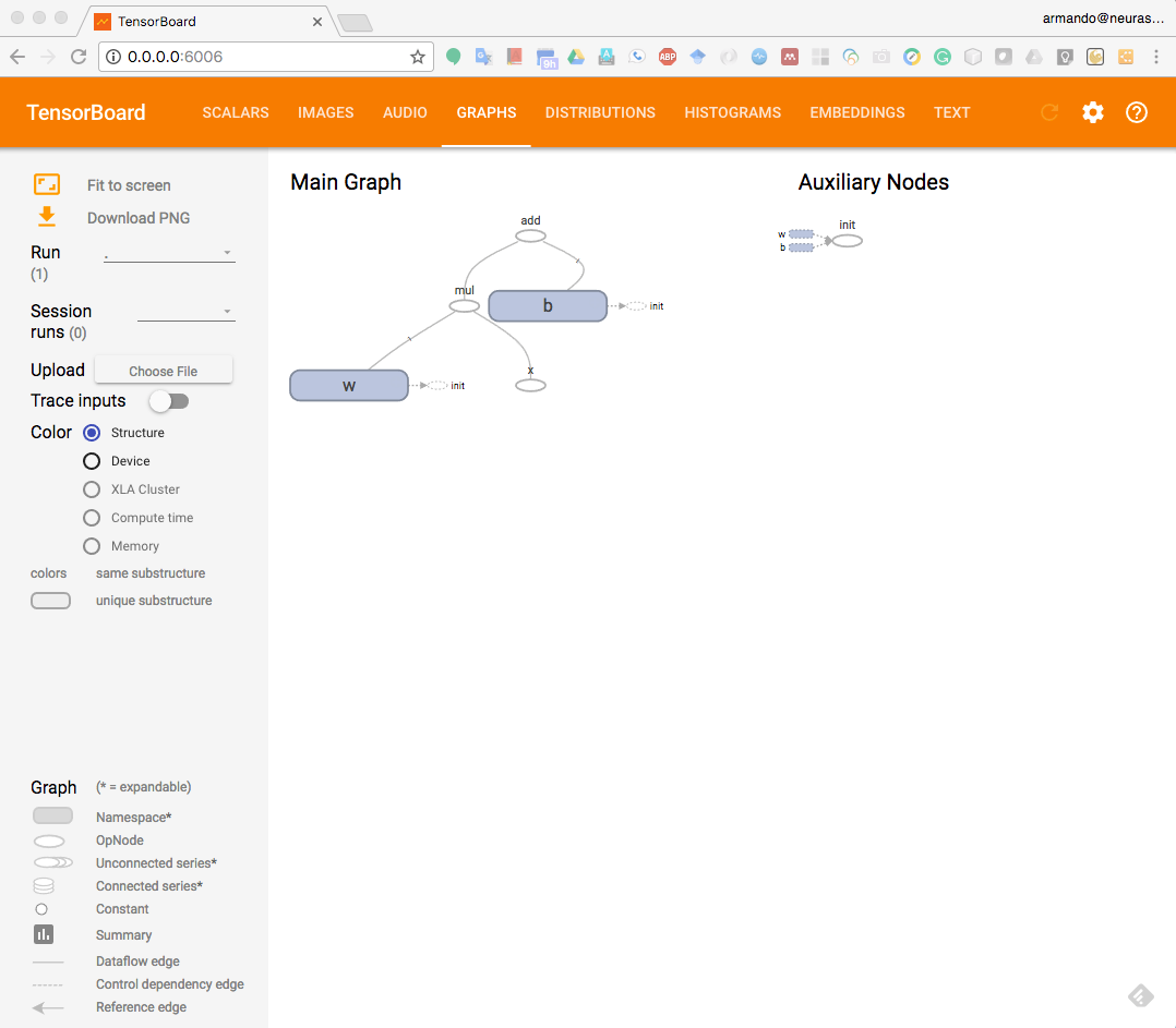
You can see that TensorBoard has visualized our first simple model as a computation graph:
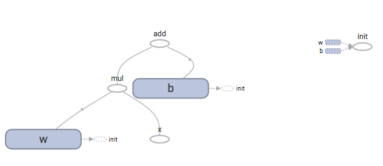
Let's now try to understand how TensorBoard works in detail.
TensorBoard details
TensorBoard works by reading log files generated by TensorFlow. Thus, we need to modify the programming model defined here to incorporate additional operation nodes that would produce the information in the logs that we want to visualize using TensorBoard. The programming model or the flow of programs with TensorBoard can be generally stated as follows:
- Create the computational graph as usual.
- Create summary nodes. Attach summary operations from the tf.summary package to the nodes that output the values that you wish to collect and analyze.
- Run the summary nodes along with running your model nodes. Generally, you would use the convenience function, tf.summary.merge_all(), to merge all the summary nodes into one summary node. Then executing this merged node would basically execute all the summary nodes. The merged summary node produces a serialized Summary ProtocolBuffers object containing the union of all the summaries.
- Write the event logs to disk by passing the Summary ProtocolBuffers object to a tf.summary.FileWriter object.
- Start TensorBoard and analyze the visualized data.
In this section, we did not create summary nodes but used TensorBoard in a very simple way. We will cover the advanced usage of TensorBoard later in this book.
Summary
In this chapter, we did a quick recap of the TensorFlow library. We learned about the TensorFlow data model elements, such as constants, variables, and placeholders, that can be used to build TensorFlow computation graphs. We learned how to create Tensors from Python objects. Tensor objects can also be generated as specific values, sequences, or random valued distributions from various library functions available in TensorFlow.
The TensorFlow programming model consists of building and executing computation graphs. The computation graphs have nodes and edges. The nodes represent operations and edges represent tensors that transfer data from one node to another. We covered how to create and execute graphs, the order of execution, and how to execute graphs on different compute devices, such as GPU and CPU. We also learned the tool to visualize the TensorFlow computation graphs, TensorBoard.
In the next chapter, we will explore some of the high-level libraries that are built on top of TensorFlow and allow us to build the models quickly.