Join our book community on Discord

https://packt.link/EarlyAccessCommunity

Convolutional Neural Networks (CNNs) are a type of deep learning model known to solve machine learning problems related to images and video, such as image classification, object detection, segmentation, and more. This is because CNNs use a special type of layer called convolutional layers, which have shared learnable parameters. The weight or parameter sharing works because the patterns to be learned in an image (such as edges or contours) are assumed to be independent of the location of the pixels in the image. Just as CNNs are applied to images, Long Short-Term Memory (LSTM) networks – which are a type of Recurrent Neural Network (RNN) – prove to be extremely effective at solving machine learning problems related to sequential data. An example of sequential data could be text. For example, in a sentence, each word is dependent on the previous word(s). LSTM models are meant to model such sequential dependencies.

These two different types of networks – CNNs and LSTMs – can be cascaded to form a hybrid model that takes in images or video and outputs text. One well-known application of such a hybrid model is image captioning, where the model takes in an image and outputs a plausible textual description of the image. Since 2010, machine learning has been used to perform the task of image captioning [2.1].

However, neural networks were first successfully used for this task in around 2014/2015 [2.2]. Ever since, image captioning has been actively researched. With significant improvements each year, this deep learning application can become useful for real-world applications such as auto-generating alt-text in websites to make them more accessible for the visually impaired.

This chapter first discusses the architecture of such a hybrid model, along with the related implementational details in PyTorch, and at the end of the chapter, we will build an image captioning system from scratch using PyTorch. This chapter covers the following topics:

• Building a neural network with CNNs and LSTMs
• Building an image caption generator using PyTorch

Building a neural network with CNNs and LSTMs

A CNN-LSTM network architecture consists of a convolutional layer(s) for extracting features from the input data (image), followed by an LSTM layer(s) to perform sequential predictions. This kind of model is both spatially and temporally deep. The convolutional part of the model is often used as an encoder that takes in an input image and outputs high-dimensional features or embeddings.

In practice, the CNN used for these hybrid networks is often pre-trained on, say, an image classification task. The last hidden layer of the pre-trained CNN model is then used as an input to the LSTM component, which is used as a decoder to generate text.

When we are dealing with textual data, we need to transform the words and other symbols (punctuation, identifiers, and more) – together referred to as tokens – into numbers. We do so by representing each token in the text with a unique corresponding number. In the following sub-section, we will demonstrate an example of text encoding.

Text encoding demo

Let's assume we're building a machine learning model with textual data; say, for example, that our text is as follows:

<start> PyTorch is a deep learning library. <end>

Then, we would map each of these words/tokens to numbers, as follows:

<start> : 0
PyTorch : 1
is : 2
a : 3
deep : 4
learning : 5
library : 6
. : 7
<end> : 8

Once we have the mapping, we can represent this sentence numerically as a list of numbers:

<start> PyTorch is a deep learning library. <end> -> [0, 1, 2, 3, 4, 5, 6, 7, 8]

Also, for example, <start> PyTorch is deep. <end> would be encoded as -> [0, 1, 2, 4, 7, 8] and so on. This mapping, in general, is referred to as vocabulary, and building a vocabulary is a crucial part of most text-related machine learning problems.

The LSTM model, which acts as the decoder, takes in a CNN embedding as input at t=0. Then, each LSTM cell makes a token prediction at each time-step, which is fed as the input to the next LSTM cell. The overall architecture thus generated can be visualized as shown in the following diagram:

The demonstrated architecture is suitable for the image captioning task. If instead of just having a single image we had a sequence of images (say, in a video) as the input to the CNN layer, then we would include the CNN embedding as the LSTM cell input at each time-step, not just at t=0. This kind of architecture would be useful for applications such as activity recognition or video description.

In the next section, we will implement an image captioning system in PyTorch that includes building a hybrid model architecture as well as data loading, preprocessing, model training, and model evaluation pipelines.

Building an image caption generator using PyTorch

For this exercise, we will be using the Common Objects in Context (COCO) dataset [2.3] , which is a large-scale object detection, segmentation, and captioning dataset.

This dataset consists of over 200,000 labeled images with five captions for each image. The COCO dataset emerged in 2014 and has helped significantly in the advancement of object recognition-related computer vision tasks. It stands as one of the most commonly used datasets for benchmarking tasks such as object detection, object segmentation, instance segmentation, and image captioning.

In this exercise, we will use PyTorch to train a CNN-LSTM model on this dataset and use the trained model to generate captions for unseen samples. Before we do that, though, there are a few pre-requisites that we need to take care of .

Note

We will be referring to only the important snippets of code for illustration purposes. The full exercise code can be found in our github repository [2.4]

Downloading the image captioning datasets

Before we begin building the image captioning system, we need to download the required datasets. If you do not have the datasets downloaded, then run the following script with the help of Jupyter Notebook. This should help with downloading the datasets locally.

Note

We are using a slightly older version of the dataset as it is slightly smaller in size, enabling us to get the results faster.

The training and validation datasets are 13 GB and 6 GB in size, respectively. Downloading and extracting the dataset files, as well as cleaning and processing them, might take a while. A good idea is to execute these steps as follows and let them finish overnight:

# download images and annotations to the data directory
!wget http://msvocds.blob.core.windows.net/annotations-1-0-3/captions_train-val2014.zip -P ./data_dir/
!wget http://images.cocodataset.org/zips/train2014.zip -P ./data_dir/
!wget http://images.cocodataset.org/zips/val2014.zip -P ./data_dir/
# extract zipped images and annotations and remove the zip files
!unzip ./data_dir/captions_train-val2014.zip -d ./data_dir/
!rm ./data_dir/captions_train-val2014.zip
!unzip ./data_dir/train2014.zip -d ./data_dir/
!rm ./data_dir/train2014.zip
!unzip ./data_dir/val2014.zip -d ./data_dir/
!rm ./data_dir/val2014.zip

You should see the following output:

This step basically creates a data folder (./data_dir), downloads the zipped images and annotation files, and extracts them inside the data folder.

Preprocessing caption (text) data

The downloaded image captioning datasets consist of both text (captions) and images. In this section, we will preprocess the text data to make it usable for our CNN-LSTM model. The exercise is laid out as a sequence of steps. The first three steps are focused on processing the text data:

1. For this exercise, we will need to import a few dependencies. Some of the crucial modules we will import for this chapter are as follows:

import nltk
from pycocotools.coco import COCO
import torch.utils.data as data
import torchvision.models as models
import torchvision.transforms as transforms
from torch.nn.utils.rnn import pack_padded_sequence

nltk is the natural language toolkit, which will be helpful in building our vocabulary, while pycocotools is a helper tool to work with the COCO dataset. The various Torch modules we have imported here have already been discussed in the previous chapter, except the last one – that is, pack_padded_sequence. This function will be useful to transform sentences with variable lengths (number of words) into fixed-length sentences by applying padding.

Besides importing the nltk library, we will also need to download its punkt tokenizer model, as follows:

nltk.download('punkt')

This will enable us to tokenize given text into constituent words.

1. Next, we build the vocabulary – that is, a dictionary that can convert actual textual tokens (such as words) into numeric tokens. This step is essential for most text-related tasks: :

def build_vocabulary(json, threshold):
    """Build a vocab wrapper."""
    coco = COCO(json)
    counter = Counter()
    ids = coco.anns.keys()
    for i, id in enumerate(ids):
        caption = str(coco.anns[id]['caption'])
        tokens = nltk.tokenize.word_tokenize(caption.lower())
        counter.update(tokens)
        if (i+1) % 1000 == 0:
            print("[{}/{}] Tokenized the captions.".format(i+1, len(ids)))

First, inside the vocabulary builder function, JSON text annotations are loaded, and individual words in the annotation/caption are tokenized or converted into numbers and stored in a counter.

Then, tokens with fewer than a certain number of occurrences are discarded, and the remaining tokens are added to a vocabulary object beside some wildcard tokens – start (of the sentence), end, unknown_word, and padding tokens, as follows:

    # If word freq < 'thres', then word is discarded.
    tokens = [token for token, cnt in counter.items() if cnt >= threshold]
    # Create vocab wrapper + add special tokens.
    vocab = Vocab()
    vocab.add_token('<pad>')
    vocab.add_token('<start>')
    vocab.add_token('<end>')
    vocab.add_token('<unk>')
    # Add words to vocab.
    for i, token in enumerate(tokens):
        vocab.add_token(token)
    return vocab

Finally, using the vocabulary builder function, a vocabulary object vocab is created and saved locally for further reuse, as shown in the following code:

vocab = build_vocabulary(json='data_dir/annotations/captions_train2014.json', threshold=4)
vocab_path = './data_dir/vocabulary.pkl'
with open(vocab_path, 'wb') as f:
    pickle.dump(vocab, f)
print("Total vocabulary size: {}".format(len(vocab)))
print("Saved the vocabulary wrapper to '{}'".format(vocab_path))

The output for this is as follows:

Once we have built the vocabulary, we can deal with the textual data by transforming it into numbers at runtime.

Preprocessing image data

After downloading the data and building the vocabulary for the text captions, we need to perform some preprocessing for the image data.

Because the images in the dataset can come in various sizes or shapes, we need to reshape all the images to a fixed shape so that they can be inputted to the first layer of our CNN model, as follows:

def reshape_images(image_path, output_path, shape):
    images = os.listdir(image_path)
    num_im = len(images)
    for i, im in enumerate(images):
        with open(os.path.join(image_path, im), 'r+b') as f:
            with Image.open(f) as image:
                image = reshape_image(image, shape)
                image.save(os.path.join(output_path, im), image.format)
        if (i+1) % 100 == 0:
            print ("[{}/{}] Resized the images and saved into '{}'.".format(i+1, num_im, output_path))
reshape_images(image_path, output_path, image_shape)

The output for this will be as follows:

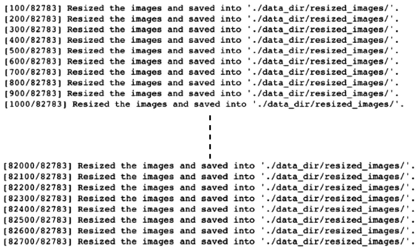
We have reshaped all the images to 256 X 256 pixels, which makes them compatible with our CNN model architecture.

Defining the image captioning data loader

We have already downloaded and preprocessed the image captioning data. Now it is time to cast this data as a PyTorch dataset object. This dataset object can subsequently be used to define a PyTorch data loader object, which we will use in our training loop to fetch batches of data as follows:

1. Now, we will implement our own custom Dataset module and a custom data loader:

class CustomCocoDataset(data.Dataset):
    """COCO Dataset compatible with torch.utils.data.DataLoader."""
    def __init__(self, data_path, coco_json_path, vocabulary, transform=None):
        """Set path for images, texts and vocab wrapper.
        
        Args:
            data_path: image directory.
            coco_json_path: coco annotation file path.
            vocabulary: vocabulary wrapper.
            transform: image transformer.
        """
        ...
    def __getitem__(self, idx):
        """Returns one data sample (X, y)."""
        ...
        return image, ground_truth
    def __len__(self):
        return len(self.indices)

First, in order to define our custom PyTorch Dataset object, we have defined our own __init__, __get_item__, and __len__ methods for instantiation, fetching items, and returning the size of the dataset, respectively.

1. Next, we define collate_function, which returns mini batches of data in the form of X, y, as follows:

def collate_function(data_batch):
    """Creates mini-batches of data
    We build custom collate function rather than using standard collate function,
    because padding is not supported in the standard version.
    Args:
        data: list of (image, caption)tuples.
            - image: tensor of shape (3, 256, 256).
            - caption: tensor of shape (:); variable length.
    Returns:
        images: tensor of size (batch_size, 3, 256, 256).
        targets: tensor of size (batch_size, padded_length).
        lengths: list.
    """
    ...       
    return imgs, tgts, cap_lens

Usually, we would not need to write our own collate function, but we do so to deal with variable-length sentences so that when the length of a sentence (say, k) is less than the fixed length, n, then we need to pad the n-k tokens with padding tokens using the pack_padded_sequence function.

1. Finally, we will implement the get_loader function, which returns a custom data loader for the COCO dataset in the following code:

def get_loader(data_path, coco_json_path, vocabulary, transform, batch_size, shuffle):
    # COCO dataset
    coco_dataset = CustomCocoDataset(data_path=data_path,
                       coco_json_path=coco_json_path,
                       vocabulary=vocabulary,
                       transform=transform)
    custom_data_loader = torch.utils.data.DataLoader(dataset=coco_dataset, batch_size=batch_size, shuffle=shuffle,  collate_fn=collate_function)
    return custom_data_loader

During the training loop, this function will be extremely useful and efficient in fetching mini batches of data.

This completes the work needed to set up the data pipeline for model training. We will now work toward the actual model itself.

Defining the CNN-LSTM model

Now that we have set up our data pipeline, we will define the model architecture as per the description in Figure 2.1, as follows:

class CNNModel(nn.Module):
    def __init__(self, embedding_size):
        """Load pretrained ResNet-152 & replace last fully connected layer."""
        super(CNNModel, self).__init__()
        resnet = models.resnet152(pretrained=True)
        module_list = list(resnet.children())[:-1]
      # delete last fully connected layer.
        self.resnet_module = nn.Sequential(*module_list)
        self.linear_layer = nn.Linear(resnet.fc.in_features, embedding_size)
        self.batch_norm = nn.BatchNorm1d(embedding_size, momentum=0.01)
            def forward(self, input_images):
        """Extract feats from images."""
        with torch.no_grad():
            resnet_features = self.resnet_module(input_images)
        resnet_features = resnet_features.reshape(resnet_features.size(0), -1)
        final_features = self.batch_norm(self.linear_layer(resnet_features))
        return final_features

We have defined two sub-models – that is, a CNN model and an RNN model. For the CNN part, we use a pre-trained CNN model available under the PyTorch models repository: the ResNet 152 architecture. While we will learn more about ResNet in detail in the next chapter, this deep CNN model with 152 layers is pre-trained on the ImageNet dataset [2.5] . The ImageNet dataset contains over 1.4 million RGB images labeled over 1,000 classes. These 1,000 classes belong to categories such as plants, animals, food, sports, and more.

We remove the last layer of this pre-trained ResNet model and replace it with a fully- connected layer followed by a batch normalization layer.

FAQ - Why are we able to replace the fully-connected layer?

The neural network can be seen as a sequence of weight matrices starting from the weight matrix between the input layer and the first hidden layer straight up to the weight matrix between the penultimate layer and the output layer. A pre-trained model can then be seen as a sequence of nicely tuned weight matrices.

By replacing the final layer, we are essentially replacing the final weight matrix (K x 1000-dimensional, assuming K number of neurons in the penultimate layer) with a new randomly initialized weight matrix (K x 256-dimensional, where 256 is the new output size).

The batch normalization layer normalizes the fully connected layer outputs with a mean of 0 and a standard deviation of 1 across the entire batch. This is similar to the standard input data normalization that we perform using torch.transforms. Performing batch normalization helps limit the extent to which the hidden layer output values fluctuate. It also generally helps with faster learning. We can use higher learning rates because of a more uniform (0 mean, 1 standard deviation) optimization hyperplane.

Since this is the final layer of the CNN sub-model, batch normalization helps insulate the LSTM sub-model against any data shifts that the CNN might introduce. If we do not use batch-norm, then in the worst-case scenario, the CNN final layer could output values with, say, mean > 0.5 and standard deviation = 1 during training. But during inference, if for a certain image the CNN outputs values with mean < 0.5 and standard deviation = 1, then the LSTM sub-model would struggle to operate on this unforeseen data distribution.

Coming back to the fully connected layer, we introduce our own layer because we do not need the 1,000 class probabilities of the ResNet model. Instead, we want to use this model to generate an embedding vector for each image. This embedding can be thought of as a one-dimensional, numerically encoded version of a given input image. This embedding is then fed to the LSTM model.

We will explore LSTMs in detail in Chapter 4, Deep Recurrent Model Architectures. But, as we have seen in Figure 2.1, the LSTM layer takes in the embedding vectors as input and outputs a sequence of words that should ideally describe the image from which the embedding was generated:

class LSTMModel(nn.Module):
    def __init__(self, embedding_size, hidden_layer_size, vocabulary_size, num_layers, max_seq_len=20):
        ...
        self.lstm_layer = nn.LSTM(embedding_size, hidden_layer_size, num_layers, batch_first=True)
        self.linear_layer = nn.Linear(hidden_layer_size, vocabulary_size)
        ...
        
    def forward(self, input_features, capts, lens):
        ...
        hidden_variables, _ = self.lstm_layer(lstm_input)
        model_outputs = self.linear_layer(hidden_variables[0])
        return model_outputs

The LSTM model consists of an LSTM layer followed by a fully connected linear layer. The LSTM layer is a recurrent layer, which can be imagined as LSTM cells unfolded along the time dimension, forming a temporal sequence of LSTM cells. For our use case, these cells will output word prediction probabilities at each time-step and the word with the highest probability is appended to the output sentence.

The LSTM cell at each time-step also generates an internal cell state, which is passed on as input to the LSTM cell of the next time-step. The process continues until an LSTM cell outputs an <end> token/word. The <end> token is appended to the output sentence. The completed sentence is our predicted caption for the image.

Note that we also specify the maximum allowed sequence length as 20 under the max_seq_len variable. This will essentially mean that any sentence shorter than 20 words will have empty word tokens padded at the end and sentences longer than 20 words will be curtailed to just the first 20 words.

Why do we do it and why 20? If we truly want our LSTM to handle sentences of any length, we might want to set this variable to an extremely large value, say, 9,999 words. However, (a) not many image captions come with that many words, and (b), more importantly, if there were ever such extra-long outlier sentences, the LSTM would struggle with learning temporal patterns across such a huge number of time-steps.

We know that LSTMs are better than RNNs at dealing with longer sequences; however, it is difficult to retain memory across such sequence lengths. We choose 20 as a reasonable number given the usual image caption lengths and the maximum length of captions we would like our model to generate.

Both the LSTM layer and the linear layer objects in the previous code are derived from nn.module and we define the __init__ and forward methods to construct the model and run a forward pass through the model, respectively. For the LSTM model, we additionally implement a sample method, as shown in the following code, which will be useful for generating captions for a given image:

    def sample(self, input_features, lstm_states=None):
        """Generate caps for feats with greedy search."""
        sampled_indices = []
        ...
        for i in range(self.max_seq_len):
...
            sampled_indices.append(predicted_outputs)
            ...
        sampled_indices = torch.stack(sampled_indices, 1)
        return sampled_indices

The sample method makes use of greedy search to generate sentences; that is, it chooses the sequence with the highest overall probability.

This brings us to the end of the image captioning model definition step. We are now all set to train this model.

Training the CNN-LSTM model

As we have already defined the model architecture in the previous section, we will now train the CNN-LSTM model. Let's examine the details of this step one by one:

1. First, we define the device. If there is a GPU available, use it for training; otherwise, use the CPU:

# Device configuration device = torch.device('cuda' if torch.cuda.is_available() else 'cpu')

Although we have already reshaped all the images to a fixed shape, (256, 256), that is not enough. We still need to normalize the data.

FAQ - Why do we need to normalize the data?

Normalization is important because different data dimensions might have different distributions, which might skew the overall optimization space and lead to inefficient gradient descent (think of an ellipse versus a circle).

1. We will use PyTorch's transform module to normalize the input image pixel values:

# Image pre-processing, normalization for pretrained resnet
transform = transforms.Compose([
    transforms.RandomCrop(224),
    transforms.RandomHorizontalFlip(),
    transforms.ToTensor(),
    transforms.Normalize((0.485, 0.456, 0.406),
                         (0.229, 0.224, 0.225))])

Furthermore, we augment the available dataset.

FAQ - Why do we need data augmentation?

Augmentation helps not only in generating larger volumes of training data but also in making the model robust against potential variations in input data.

Using PyTorch's transform module, we implement two data augmentation techniques here:

i) Random cropping, resulting in the reduction of the image size from (256, 256) to (224, 224).

ii) Horizontal flipping of the images.

1. Next, we load the vocabulary that we built in the Preprocessing caption (text) data section. We also initialize the data loader using the get_loader function defined in the Defining the image captioning data loader section:

# Load vocab wrapper
with open('data_dir/vocabulary.pkl', 'rb') as f:
    vocabulary = pickle.load(f)
    
# Instantiate data loader
custom_data_loader = get_loader('data_dir/resized_images', 'data_dir/annotations/captions_train2014.json', vocabulary,
                         transform, 128,
                         shuffle=True)

1. Next, we arrive at the main section of this step, where we instantiate the CNN and LSTM models in the form of encoder and decoder models. Furthermore, we also define the loss function – cross entropy loss – and the optimization schedule – the Adam optimizer – as follows:

# Build models
encoder_model = CNNModel(256).to(device)
decoder_model = LSTMModel(256, 512, len(vocabulary), 1).to(device)
    
# Loss & optimizer
loss_criterion = nn.CrossEntropyLoss()
parameters = list(decoder_model.parameters()) + list(encoder_model.linear_layer.parameters()) + list(encoder_model.batch_norm.parameters())
optimizer = torch.optim.Adam(parameters, lr=0.001)

As discussed in Chapter 1, Overview of Deep Learning Using PyTorch, Adam is possibly the best choice for an optimization schedule when dealing with sparse data. Here, we are dealing with both images and text – perfect examples of sparse data because not all pixels contain useful information and numericized/vectorized text is a sparse matrix in itself.

1. Finally, we run the training loop (for five epochs) where we use the data loader to fetch a mini batch of the COCO dataset, run a forward pass with the mini batch through the encoder and decoder networks, and finally, tune the parameters of the CNN-LSTM model using backpropagation (backpropagation through time, for the LSTM network):

for epoch in range(5):
    for i, (imgs, caps, lens) in enumerate(custom_data_loader):
        tgts = pack_padded_sequence(caps, lens, batch_first=True)[0]
        # Forward pass, backward propagation
        feats = encoder_model(imgs)
        outputs = decoder_model(feats, caps, lens)
        loss = loss_criterion(outputs, tgts)
        decoder_model.zero_grad()
        encoder_model.zero_grad()
        loss.backward()
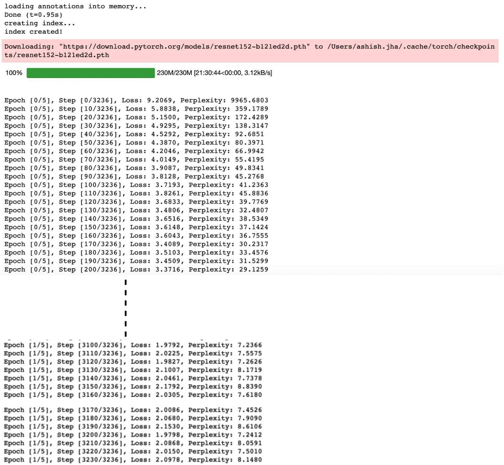
        optimizer.step()

Every 1,000 iterations into the training loop, we save a model checkpoint. For demonstration purposes, we have run the training for just two epochs, as follows:

        # Log training steps
        if i % 10 == 0:
            print('Epoch [{}/{}], Step [{}/{}], Loss: {:.4f}, Perplexity: {:5.4f}'
                  .format(epoch, 5, i, total_num_steps, loss.item(), np.exp(loss.item())))
        # Save model checkpoints
        if (i+1) % 1000 == 0:
            torch.save(decoder_model.state_dict(), os.path.join(
                'models_dir/', 'decoder-{}-{}.ckpt'.format(epoch+1, i+1)))
            torch.save(encoder_model.state_dict(), os.path.join(
                'models_dir/', 'encoder-{}-{}.ckpt'.format(epoch+1, i+1)))

The output will be as follows:

Generating image captions using the trained model

We have trained an image captioning model in the previous section. In this section, we will use the trained model to generate captions for images previously unseen by the model:

1. We have stored a sample image, sample.jpg, to run inference on. We define a function to load the image and reshape it to (224, 224) pixels. Then , we define the transformation module to normalize the image pixels, as follows:

image_file_path = 'sample.jpg'
# Device config
device = torch.device('cuda' if torch.cuda.is_available() else 'cpu')
def load_image(image_file_path, transform=None):
    img = Image.open(image_file_path).convert('RGB')
    img = img.resize([224, 224], Image.LANCZOS)
    if transform is not None:
        img = transform(img).unsqueeze(0)
    return img
# Image pre-processing
transform = transforms.Compose([
    transforms.ToTensor(),
    transforms.Normalize((0.485, 0.456, 0.406),
                         (0.229, 0.224, 0.225))])

1. Next, we load the vocabulary and instantiate the encoder and decoder models:

# Load vocab wrapper
with open('data_dir/vocabulary.pkl', 'rb') as f:
    vocabulary = pickle.load(f)
# Build models
encoder_model = CNNModel(256).eval()  # eval mode (batchnorm uses moving mean/variance)
decoder_model = LSTMModel(256, 512, len(vocabulary), 1)
encoder_model = encoder_model.to(device)
decoder_model = decoder_model.to(device)

1. Once we have the model scaffold ready, we will use the latest saved checkpoint from the two epochs of training to set the model parameters:

# Load trained model params
encoder_model.load_state_dict(torch.load('models_dir/encoder-2-3000.ckpt'))
decoder_model.load_state_dict(torch.load('models_dir/decoder-2-3000.ckpt'))

After this point, the model is ready to use for inference.

1. Next, we load the image and run model-inference – that is, first we use the encoder model to generate an embedding from the image, and then we feed the embedding to the decoder network to generate sequences, as follows:

# Prepare image
img = load_image(image_file_path, transform)
img_tensor = img.to(device)
# Generate caption text from image
feat = encoder_model(img_tensor)
sampled_indices = decoder_model.sample(feat)
sampled_indices = sampled_indices[0].cpu().numpy()
          # (1, max_seq_length) -> (max_seq_length)

1. At this stage, the caption predictions are still in the form of numeric tokens. We need to convert the numeric tokens into actual text using the vocabulary in reverse:

# Convert numeric tokens to text tokens
predicted_caption = []
for token_index in sampled_indices:
    word = vocabulary.i2w[token_index]
    predicted_caption.append(word)
    if word == '<end>':
        break
predicted_sentence = ' '.join(predicted_caption)

1. Once we have transformed our output into text, we can visualize both the image as well as the generated caption:

# Print image & generated caption text
print (predicted_sentence)
img = Image.open(image_file_path)
plt.imshow(np.asarray(img))

The output will be as follows:

It seems that although the model is not absolutely perfect, within two epochs, it is already trained well enough to generate sensible captions.

Summary

This chapter discussed the concept of combining a CNN model and an LSTM model in an encoder-decoder framework, jointly training them, and using the combined model to generate captions for an image.

We have used CNNs both in this and the previous chapter's exercises.

In the next chapter, we will take a deeper look at the gamut of different CNN architectures developed over the years, how each of them is uniquely useful, and how they can be easily implemented using PyTorch.